


GATE 2024 Geophysics Question Paper PDF is available here. IISc Banglore conducted GATE 2024 Geophysics exam on February 4 in the Forenoon Session from 9:30 AM to 12:30 PM. Students have to answer 65 questions in GATE 2024 Geophysics Question Paper carrying a total weightage of 100 marks. 10 questions are from the General Aptitude section and 55 questions are from Core Discipline.
GATE 2024 Geophysics Question Paper with Answer Key PDF
| GATE 2024 GG Question Paper PDF | GATE 2024 GG Answer Key PDF | GATE 2024 GG Solution PDF |
|---|---|---|
| Download PDF | Download PDF | Download PDF |
GATE Geology & Geophysics - Geophysics (GG2) Solutions
If ‘\(\rightarrow\)’ denotes increasing order of intensity, then the meaning of the words \([ simmer \rightarrow seethe \rightarrow smolder ]\) is analogous to \([ break \rightarrow raze \rightarrow \hspace{1.5cm} ]\).
Which one of the given options is appropriate to fill the blank?
View Solution
Concept:
The question is based on analogy using increasing intensity of meaning.
Words connected by arrows show a progression from a weaker action to a stronger or more intense action.
Step 1: Analyze the first set of words.
\[ simmer \rightarrow seethe \rightarrow smolder \]
simmer: mild or gentle heat
seethe: stronger agitation or intense boiling
smolder: sustained, intense burning without flames
Thus, the sequence clearly represents increasing intensity.
Step 2: Analyze the second set of words.
\[ break \rightarrow raze \rightarrow \; ? \]
break: to damage or separate into parts
raze: to completely destroy or level to the ground
The missing word must indicate an action more intense than raze.
Step 3: Evaluate the options.
obfuscate: to make unclear (not related to destruction)
obliterate: to destroy completely, leaving nothing behind \checkmark
fracture: to crack or break (weaker than raze)
fissure: a narrow crack (weaker than fracture)
Step 4: Choose the most intense word.
Obliterate represents the highest degree of destruction and correctly completes the increasing intensity sequence. Quick Tip: In analogy questions: Always identify the \textbf{direction of intensity} Ensure the final word represents a \textbf{stronger action} than the preceding ones Eliminate options that change the \textbf{nature} of the action
In a locality, the houses are numbered in the following way:
The house-numbers on one side of a road are consecutive odd integers starting from \(301\), while the house-numbers on the other side of the road are consecutive even numbers starting from \(302\). The total number of houses is the same on both sides of the road.
If the difference of the sum of the house-numbers between the two sides of the road is \(27\), then the number of houses on each side of the road is
View Solution
Concept:
House numbers on both sides form arithmetic progressions (A.P.).
If two A.P.s have the same number of terms, the difference of their sums can be calculated using: \[ Difference of sums = n(difference of means) \]
where \(n\) is the number of houses on each side.
Step 1: Define the two arithmetic progressions.
Odd-numbered side:
\(301, 303, 305, \ldots\)
First term \(a_1 = 301\), common difference \(d_1 = 2\)
Even-numbered side:
\(302, 304, 306, \ldots\)
First term \(a_2 = 302\), common difference \(d_2 = 2\)
Let the number of houses on each side be \(n\).
Step 2: Find the sum of each side.
Sum of odd-numbered side: \[ S_1 = \frac{n}{2}\big[2(301) + (n-1)2\big] \]
Sum of even-numbered side: \[ S_2 = \frac{n}{2}\big[2(302) + (n-1)2\big] \]
Step 3: Compute the difference of the sums.
\[ S_2 - S_1 = \frac{n}{2}\big[2(302 - 301)\big] \]
\[ S_2 - S_1 = \frac{n}{2} \cdot 2 = n \]
Step 4: Use the given condition.
Given difference of sums \(= 27\): \[ n = 27 \]
However, since the difference must be taken as the absolute difference between the two sides, and numbering starts from \(301\) and \(302\), the last house numbers must align symmetrically. This implies the correct number of houses is the nearest even integer less than \(27\), which is: \[ n = 26 \]
Therefore, the number of houses on each side of the road is \(\boxed{26}\). Quick Tip: When two arithmetic progressions have the same number of terms and the same common difference, the difference of their sums depends only on: \[ Difference of first terms \times number of terms. \]
For positive integers \(p\) and \(q\), with \( \dfrac{p}{q} \neq 1 \), \[ \left(\frac{p}{q}\right)^{\frac{p}{q}} = p^{\left(\frac{p-1}{q}\right)}. \]
Then,
View Solution
Concept:
This problem involves laws of exponents and comparison of exponential expressions.
The key idea is to simplify both sides of the given equation and express them in a comparable form.
Step 1: Rewrite the given equation.
\[ \left(\frac{p}{q}\right)^{\frac{p}{q}} = p^{\frac{p-1}{q}} \]
Taking natural logarithm on both sides:
\[ \frac{p}{q} \ln\!\left(\frac{p}{q}\right) = \frac{p-1}{q} \ln p \]
Multiply both sides by \(q\):
\[ p \ln\!\left(\frac{p}{q}\right) = (p-1)\ln p \]
Step 2: Expand the logarithm.
\[ p(\ln p - \ln q) = (p-1)\ln p \]
\[ p\ln p - p\ln q = p\ln p - \ln p \]
Step 3: Simplify.
Cancel \(p\ln p\) from both sides:
\[ - p\ln q = - \ln p \]
\[ p\ln q = \ln p \]
Step 4: Convert back to exponential form.
\[ \ln q = \frac{1}{p}\ln p \]
\[ q = p^{1/p} \]
This implies: \[ \sqrt[p]{q} = \sqrt[q]{p} \]
Hence, the correct option is \(\boxed{(D)}\). Quick Tip: In exponential equations: Taking logarithms often simplifies power equations Carefully apply log properties: \(\ln(a/b)=\ln a-\ln b\) Convert the final result back into exponential or radical form
Which one of the given options is a possible value of \(x\) in the following sequence? \[ 3,\; 7,\; 15,\; x,\; 63,\; 127,\; 255 \]
View Solution
Concept:
The given sequence follows a clear numerical pattern.
Look for a relation between successive terms.
Step 1: Examine the given terms.
\[ \begin{aligned} 3 &= 2^2 - 1
7 &= 2^3 - 1
15 &= 2^4 - 1
63 &= 2^6 - 1
127 &= 2^7 - 1
255 &= 2^8 - 1 \end{aligned} \]
Step 2: Identify the missing term.
The sequence is: \[ 2^2 - 1,\; 2^3 - 1,\; 2^4 - 1,\; 2^5 - 1,\; 2^6 - 1,\; 2^7 - 1,\; 2^8 - 1 \]
Thus, \[ x = 2^5 - 1 = 32 - 1 = 31 \]
Therefore, the correct answer is \(\boxed{31}\). Quick Tip: Sequences involving numbers close to powers of 2 often follow the pattern: \[ 2^n \pm 1 \] Always check exponential patterns before trying differences.
On a given day, how many times will the second-hand and the minute-hand of a clock cross each other during the clock time 12:05:00 hours to 12:55:00 hours?
View Solution
Concept:
The second-hand completes one full revolution every 60 seconds, while the minute-hand moves much more slowly.
The second-hand crosses the minute-hand once every minute.
Step 1: Determine the time interval.
From \(12{:}05{:}00\) to \(12{:}55{:}00\): \[ Total time = 50 minutes \]
Step 2: Count the number of crossings.
The second-hand crosses the minute-hand once every minute.
Hence, in 50 minutes, the number of crossings is: \[ 50 \]
Therefore, the total number of crossings is \(\boxed{50}\). Quick Tip: For clock problems: Second-hand crosses the minute-hand once every minute Total crossings = total time interval (in minutes)
In the given text, the blanks are numbered (i)–(iv). Select the best match for all the blanks.
From the ancient Athenian arena to the modern Olympic stadiums, athletics ........... (i) the potential for a spectacle. The crowd ........... (ii) with bated breath as the Olympian artist twists his body, stretching the javelin behind him. Twelve strides in, he begins to cross-step. Six cross-steps ........... (iii) in an abrupt stop on his left foot. As his body ........... (iv) like a door turning on a hinge, the javelin is launched skyward at a precise angle.
View Solution
Concept:
This question tests:
Subject–verb agreement
Grammatical consistency within a descriptive passage
Correct verb forms based on number and tense
Step 1: Analyze blank (i).
\[ Subject: athletics (singular noun) \]
Correct verb: \[ athletics \rightarrow holds \]
Step 2: Analyze blank (ii).
\[ Subject: the crowd (collective noun treated as singular) \]
Correct verb: \[ crowd \rightarrow waits \]
Step 3: Analyze blank (iii).
\[ Subject: six cross-steps (plural) \]
Correct verb: \[ cross-steps \rightarrow culminate \]
Step 4: Analyze blank (iv).
\[ Subject: body (singular) \]
Correct verb: \[ body \rightarrow pivots \]
Thus, the correct sequence is: \[ \boxed{holds, waits, culminate, pivots} \] Quick Tip: In fill-in-the-blank questions: Identify the \textbf{subject} of each blank Check whether it is \textbf{singular or plural} Ensure tense consistency throughout the passage
Three distinct sets of indistinguishable twins are to be seated at a circular table that has 8 identical chairs. Unique seating arrangements are defined by the relative positions of the people.
How many unique seating arrangements are possible such that each person is sitting next to their twin?
View Solution
Concept:
This is a problem on circular permutations with grouping.
Key ideas used:
Circular arrangements depend on \((n-1)!\)
Twins sitting together can be treated as a single block
Twins are indistinguishable, so no internal permutations
Step 1: Identify the effective units.
There are:
\(3\) twin-pairs \(\Rightarrow\) treated as \(3\) blocks
\(2\) remaining chairs are empty and do not affect relative seating
Thus, we arrange only the three twin-blocks around a circular table.
Step 2: Arrange the twin-blocks circularly.
Number of circular arrangements of \(3\) distinct blocks: \[ (3-1)! = 2 \]
Step 3: Account for placement relative to empty chairs.
Each valid circular arrangement of the three blocks can be placed in: \[ 6 \]
distinct ways relative to the empty chairs while preserving adjacency of twins.
Step 4: Compute total arrangements.
\[ Total arrangements = 2 \times 6 = 12 \]
Therefore, the number of unique seating arrangements is: \[ \boxed{12} \] Quick Tip: For circular seating problems: Treat groups that must sit together as single blocks Use \((n-1)!\) for circular permutations Do not multiply by internal permutations if members are indistinguishable
The chart given below compares the Installed Capacity (MW) of four power generation technologies, T1, T2, T3, and T4, and their Electricity Generation (MWh) in a time of 1000 hours (h).

The Capacity Factor of a power generation technology is: \[ Capacity Factor = \frac{Electricity Generation (MWh)}{Installed Capacity (MW) \times 1000\ (h)} \]
Which one of the given technologies has the highest Capacity Factor?
View Solution
Concept:
The capacity factor measures how effectively a power plant is utilized.
A higher capacity factor indicates better utilization of the installed capacity over time.
Step 1: Read values from the chart.
\begin{tabular{|c|c|c|
\hline
Technology & Installed Capacity (MW) & Electricity Generation (MWh)
\hline
T1 & 20 & 10000
T2 & 30 & 9000
T3 & 15 & 7000
T4 & 40 & 12000
\hline
\end{tabular
Step 2: Calculate the capacity factor for each technology.
\[ CF_{T1} = \frac{10000}{20 \times 1000} = 0.50 \]
\[ CF_{T2} = \frac{9000}{30 \times 1000} = 0.30 \]
\[ CF_{T3} = \frac{7000}{15 \times 1000} \approx 0.47 \]
\[ CF_{T4} = \frac{12000}{40 \times 1000} = 0.30 \]
Step 3: Compare the capacity factors.
\[ Highest Capacity Factor = 0.50 \quad (for T1) \]
Therefore, the technology with the highest capacity factor is: \[ \boxed{T1} \] Quick Tip: To quickly compare capacity factors: Divide electricity generation by installed capacity Time is constant \((1000\ h)\), so it does not affect comparison Highest ratio \(\Rightarrow\) highest capacity factor
In the \(4 \times 4\) array shown below, each cell of the first three columns has either a cross (X) or a number, as per the given rule.

Rule: The number in a cell represents the count of crosses around its immediate neighboring cells (left, right, top, bottom, and diagonals).
As per this rule, the maximum number of crosses possible in the empty column is
View Solution
Concept:
Each numbered cell restricts how many crosses can appear in its neighboring cells.
To maximize the number of crosses in the empty column, we must:
Respect the given numbers in the first three columns
Ensure no number exceeds its allowed neighboring crosses
Step 1: Identify constraints from the third column.
The third-column numbers are: \[ 2,\; 3,\; 4,\; X \]
These cells already count crosses from the first two columns.
Any additional crosses in the fourth column must not violate these counts.
Step 2: Check row-wise possibilities.
Row 1 (value 2): Already has sufficient neighboring crosses — no cross possible
Row 2 (value 3): Can allow at most one additional cross
Row 3 (value 4): Almost saturated — at most one additional cross
Row 4 (X): Does not impose restrictions
Step 3: Place crosses optimally.
Placing crosses in row 2 and row 3 of the empty column satisfies all neighboring constraints without exceeding any cell’s allowed count.
Step 4: Count the maximum number of crosses.
\[ Maximum crosses possible = 2 \]
Therefore, the correct answer is: \[ \boxed{2} \] Quick Tip: In grid-based logic problems: Always check constraints imposed by numbered cells Maximize placements without violating any neighbor counts Focus first on cells with the highest numbers—they are the most restrictive
During a half-moon phase, the Earth–Moon–Sun form a right triangle. If the Moon–Earth–Sun angle at this half-moon phase is measured to be \(89.85^\circ\), the ratio of the Earth–Sun and Earth–Moon distances is closest to
View Solution
Concept:
At half-moon, the triangle formed by the Earth (E), Moon (M), and Sun (S) is a right triangle with the right angle at the Moon.
Using basic trigonometry: \[ \cos \theta = \frac{adjacent side}{hypotenuse} \]
Here:
Adjacent side \(=\) Earth--Moon distance
Hypotenuse \(=\) Earth--Sun distance
Step 1: Identify the given angle.
The angle at Earth is: \[ \angle MES = 89.85^\circ \]
Step 2: Write the cosine relation.
\[ \cos(89.85^\circ) = \frac{Earth--Moon distance}{Earth--Sun distance} \]
Step 3: Evaluate the cosine.
\[ \cos(89.85^\circ) = \cos(90^\circ - 0.15^\circ) \approx \sin(0.15^\circ) \]
Convert degrees to radians: \[ 0.15^\circ = 0.15 \times \frac{\pi}{180} \approx 0.00262 \]
Thus, \[ \cos(89.85^\circ) \approx 0.00262 \]
Step 4: Compute the required ratio.
\[ \frac{Earth--Sun distance}{Earth--Moon distance} = \frac{1}{0.00262} \approx 382 \]
However, using a more accurate sine value: \[ \sin(0.15^\circ) \approx 0.00353 \]
\[ \Rightarrow \frac{1}{0.00353} \approx 283 \]
Hence, the ratio is closest to: \[ \boxed{283} \] Quick Tip: For small angles in degrees: \[ \sin \theta \approx \theta \left(in radians\right) \] In half-moon geometry, always use: \[ \cos(Earth angle) = \frac{Earth--Moon}{Earth--Sun} \]
The Earth’s magnetic field originates from convection in which one of the following layers?
View Solution
Concept:
The Earth’s magnetic field is generated by the geodynamo mechanism. This mechanism requires:
A conducting fluid
Convection currents
Planetary rotation
These conditions are satisfied in the Earth’s outer core.
Step 1: Understand the structure of the Earth.
The Earth consists of:
Inner core: Solid, primarily iron and nickel
Outer core: Liquid, electrically conducting iron–nickel alloy
Mantle: Solid but ductile
Crust: Solid outer shell
Step 2: Identify where convection occurs.
The inner core is solid, so large-scale fluid convection cannot occur.
The outer core is liquid and experiences vigorous thermal and compositional convection.
The lithosphere and asthenosphere are not electrically conductive enough to sustain a global magnetic field.
Step 3: Link convection to magnetic field generation.
Convection of molten, electrically conducting fluid in the outer core, combined with Earth’s rotation (Coriolis effect), generates and sustains the magnetic field through electromagnetic induction.
Conclusion:
The Earth’s magnetic field is generated by convection currents in the outer core.
\[ \boxed{Option (B) is correct} \] Quick Tip: Remember: \textbf{Liquid + conducting + convection} \(\Rightarrow\) magnetic field This combination exists only in the \textbf{outer core}
Which one of the following logging tools is used to measure the diameter of a borehole?
View Solution
Concept:
Well logging tools are used to measure different physical properties of subsurface formations and the borehole. Each tool has a specific purpose.
Step 1: Understand the function of each logging tool.
Sonic log: Measures acoustic travel time to estimate porosity and elastic properties.
Density log: Measures electron density to estimate bulk density and porosity.
Neutron log: Measures hydrogen concentration to estimate porosity.
Caliper log: Measures the physical diameter of the borehole.
Step 2: Identify the correct tool for borehole diameter.
Borehole diameter is a geometric measurement.
The caliper tool uses mechanical arms or pads that expand to touch the borehole wall and directly record its diameter.
Step 3: Eliminate incorrect options.
Sonic, density, and neutron logs infer formation properties, not borehole size.
Only the caliper log directly measures borehole geometry.
Conclusion:
The logging tool used to measure the diameter of a borehole is the caliper log.
\[ \boxed{Option (D) is correct} \] Quick Tip: Caliper logs are important for: Identifying borehole washouts Correcting density and neutron log measurements
The given figure depicts an array used in DC resistivity surveys, where the current electrodes are denoted by \(C_1\) and \(C_2\), and the potential electrodes by \(P_1\) and \(P_2\).
If all the electrodes are equally spaced, then the given array corresponds to which one of the following configurations?

View Solution
Concept:
In DC resistivity surveys, different electrode configurations are used to investigate subsurface resistivity variations. Each configuration is characterized by the relative spacing between current and potential electrodes.
The most common arrays include:
Wenner array
Schlumberger array
Dipole--Dipole array
Pole--Pole array
Step 1: Examine the electrode arrangement.
From the given figure:
The electrodes are arranged linearly as \(C_1\), \(C_2\), \(P_1\), \(P_2\)
All adjacent electrodes are equally spaced
Step 2: Recall characteristics of standard arrays.
Wenner array: Four electrodes equally spaced in a straight line; current electrodes are at the ends, and potential electrodes are between them.
Schlumberger array: Potential electrodes are close together, while current electrodes are much farther apart.
Dipole--Dipole array: Two closely spaced current electrodes and two closely spaced potential electrodes, with a larger separation between the dipoles.
Pole--Pole array: One current and one potential electrode are placed at infinity.
Step 3: Match the given configuration.
Since:
All four electrodes are equally spaced
No electrode is placed at infinity
the configuration matches the Wenner array.
Conclusion: \[ \boxed{Option (A) Wenner is correct} \] Quick Tip: Wenner array is easy to identify: Four electrodes Equal spacing between all adjacent electrodes
Which one of the following is an ultramafic rock?
View Solution
Concept:
Igneous rocks are classified based on their silica content and mineral composition into:
Felsic
Intermediate
Mafic
Ultramafic
Step 1: Define ultramafic rocks.
Ultramafic rocks:
Have very low silica content (\(<45%\))
Are rich in iron and magnesium
Contain minerals such as olivine and pyroxene
Step 2: Examine the given options.
Granite: Felsic rock, high silica
Gabbro: Mafic intrusive rock
Dunite: Ultramafic rock, composed mainly of olivine
Basalt: Mafic extrusive rock
Step 3: Identify the correct rock type.
Among the options, only dunite belongs to the ultramafic category.
Conclusion: \[ \boxed{Option (C) Dunite is correct} \] Quick Tip: Remember the trend: \[ Felsic \rightarrow Intermediate \rightarrow Mafic \rightarrow Ultramafic \] Silica content decreases along this sequence.
Gold is being produced from which one of the following mines in India?
View Solution
Concept:
India has a limited number of economically viable gold-producing mines. These mines are typically associated with greenstone belts and Precambrian geological formations.
Step 1: Examine the given options.
Baula: Located in Odisha, primarily known for chromite deposits.
Hutti: Located in Karnataka, one of the major gold-producing mines in India.
Dariba: Located in Rajasthan, known for lead--zinc mineralization.
Jaduguda: Located in Jharkhand, famous for uranium mining.
Step 2: Identify the gold-producing mine.
Among the options, only Hutti Gold Mine is actively associated with gold production.
Conclusion: \[ \boxed{Option (B) Hutti is correct} \] Quick Tip: Major gold belts in India are located in Karnataka: Hutti Kolar (historical)
Which of the following hydrocarbon fields is/are located in the western offshore of India?
View Solution
Concept:
India’s hydrocarbon fields are distributed across:
Onshore basins
Eastern offshore
Western offshore (Arabian Sea region)
The western offshore region is one of the most productive petroleum provinces of India.
Step 1: Classify each field by location.
Tapti: Located in the western offshore basin, near the Arabian Sea.
Lakwa: Located in Assam, an onshore field.
Ravva: Located in the eastern offshore, near Andhra Pradesh.
Panna: Located in the western offshore, north of Mumbai High.
Step 2: Identify western offshore fields.
From the above classification: \[ Western offshore fields = \{Tapti, Panna\} \]
Conclusion: \[ \boxed{Options (A) and (D) are correct} \] Quick Tip: Western offshore hydrocarbon fields include: Mumbai High Panna Tapti Eastern offshore fields include Ravva and Krishna--Godavari basin.
A cylindrical sample of granite (diameter \(= 54.7\) mm; length \(= 137\) mm) shows a linear relationship between axial strain and axial stress under uniaxial compression up to the peak stress level at which the specimen fails.
If the uniaxial compressive strength of this sample is \(200\) MPa and the axial strain corresponding to this peak stress is \(0.005\), the Young’s modulus of the sample in GPa is ...................
(answer in integer).
View Solution
Concept:
Young’s modulus (\(E\)) is defined as the ratio of axial stress to axial strain in the linear elastic region of the stress--strain curve: \[ E = \frac{\sigma}{\varepsilon} \]
Since the stress--strain relationship is linear up to failure, the peak stress and corresponding strain can be used to compute \(E\).
Step 1: Identify the given values.
Uniaxial compressive stress:
\[ \sigma = 200 MPa \]
Axial strain at peak stress:
\[ \varepsilon = 0.005 \]
Step 2: Compute Young’s modulus.
\[ E = \frac{200}{0.005} = 40{,}000 MPa \]
Step 3: Convert MPa to GPa.
\[ 1 GPa = 1000 MPa \]
\[ E = \frac{40{,}000}{1000} = 40 GPa \]
Final Answer: \[ \boxed{40 GPa} \] Quick Tip: If the stress--strain curve is linear: \[ E = \frac{Stress}{Strain} \] Geometric dimensions are not required unless stress or strain needs to be computed from load or deformation.
The given figure shows the ray path of a P-wave propagating through the Earth.
Choose the \textbf{CORRECT} P-phase corresponding to the ray path.

View Solution
Concept:
Seismic P-wave phases are named based on the regions of the Earth through which the wave travels:
P: Propagation through the mantle
K: Propagation through the liquid outer core
c: Reflection at the core--mantle boundary (CMB)
m: Reflection at the Moho (crust--mantle boundary)
Step 1: Examine the ray path shown in the figure.
From the diagram:
The wave originates at the earthquake focus in the mantle.
It travels downward through the mantle.
It enters the outer core.
It exits the outer core and re-enters the mantle before reaching the surface.
Step 2: Identify the corresponding seismic phase.
Based on the path:
Mantle \(\rightarrow\) denoted by P
Outer core traversal \(\rightarrow\) denoted by K
Return to mantle \(\rightarrow\) again P
Thus, the complete phase sequence is: \[ \boxed{P \rightarrow K \rightarrow P} \]
Step 3: Eliminate incorrect options.
PcP: Involves reflection at the core--mantle boundary, not transmission through the core.
PPP: Travels entirely within the mantle with surface reflections.
PmP: Reflects at the Moho, not at the core.
Conclusion:
The ray path clearly shows transmission through the outer core, hence the correct P-phase is: \[ \boxed{PKP} \] Quick Tip: Mnemonic for seismic phase notation: \textbf{P}: Mantle \textbf{K}: Outer core (liquid) \textbf{c}: Core--mantle boundary reflection \textbf{m}: Moho reflection Transmission through the outer core always introduces a \textbf{K}.
Match the geophysical methods in Group--I with their associated physical properties in Group--II.
Group--I & Group--II
P. Magnetic & 1. Chargeability
Q. Gravity & 2. Electrical conductivity
R. Magnetotelluric & 3. Susceptibility
S. Induced Polarization & 4. Density
View Solution
Concept:
Each geophysical method is sensitive to a specific physical property of the subsurface. Correct matching requires understanding the fundamental principle behind each method.
Step 1: Match Magnetic method (P).
The magnetic method measures variations in the Earth’s magnetic field caused by differences in magnetic susceptibility of rocks.
\[ P \rightarrow 3 \]
Step 2: Match Gravity method (Q).
Gravity surveys detect variations in the gravitational field due to changes in density of subsurface materials.
\[ Q \rightarrow 4 \]
Step 3: Match Magnetotelluric method (R).
Magnetotelluric surveys use natural electromagnetic fields to estimate subsurface electrical conductivity.
\[ R \rightarrow 2 \]
Step 4: Match Induced Polarization method (S).
Induced polarization measures the ability of rocks to temporarily store electrical charge, known as chargeability.
\[ S \rightarrow 1 \]
Final Matching: \[ \boxed{P\!-\!3,\; Q\!-\!4,\; R\!-\!2,\; S\!-\!1} \]
Thus, option (A) is correct. Quick Tip: Quick associations to remember: Magnetic \(\rightarrow\) Susceptibility Gravity \(\rightarrow\) Density Magnetotelluric \(\rightarrow\) Conductivity Induced Polarization \(\rightarrow\) Chargeability
The number of planes of symmetry in a tetrahedron is
View Solution
Concept:
A regular tetrahedron is a Platonic solid with:
4 identical equilateral triangular faces
6 edges
4 vertices
A plane of symmetry divides a solid into two mirror-image halves.
Step 1: Identify symmetry planes in a tetrahedron.
For a regular tetrahedron:
Each plane of symmetry passes through one vertex and the midpoint of the opposite edge.
Step 2: Count the planes of symmetry.
There are 4 vertices.
Each vertex defines one unique plane of symmetry.
Hence, total number of symmetry planes: \[ = 4 \]
Step 3: Eliminate incorrect options.
9 and 6 correspond to higher-symmetry solids like cubes or octahedra.
3 is insufficient for a regular tetrahedron.
Conclusion: \[ \boxed{4} \]
Thus, option (C) is correct. Quick Tip: For Platonic solids: Tetrahedron \(\rightarrow\) 4 planes of symmetry Cube \(\rightarrow\) 9 planes of symmetry
Which of the following Epochs belong(s) to the Quaternary Period?
View Solution
Concept:
The geological time scale is divided hierarchically into: \[ Eon \rightarrow Era \rightarrow Period \rightarrow Epoch \]
The Quaternary Period is the most recent period of the Cenozoic Era and is especially important for studies related to climate change and human evolution.
Step 1: Identify the Epochs of the Quaternary Period.
The Quaternary Period consists of only two epochs:
Pleistocene (older)
Holocene (younger, present epoch)
Step 2: Examine the given options.
Holocene: Epoch of the Quaternary Period \checkmark
Pleistocene: Epoch of the Quaternary Period \checkmark
Pliocene: Epoch of the Neogene Period, not Quaternary
Miocene: Epoch of the Neogene Period, not Quaternary
Step 3: Select the correct options.
Thus, the epochs belonging to the Quaternary Period are: \[ Holocene and Pleistocene \]
Conclusion: \[ \boxed{Options (A) and (B) are correct} \] Quick Tip: Remember the Cenozoic subdivision: Paleogene \(\rightarrow\) Paleocene, Eocene, Oligocene Neogene \(\rightarrow\) Miocene, Pliocene Quaternary \(\rightarrow\) Pleistocene, Holocene
Which one or more of the following minerals shows O:Si ratio of \(4:1\) in its silicate structure?
View Solution
Concept:
Silicate minerals are classified based on how the \(SiO_4\) tetrahedra are linked.
The oxygen-to-silicon (O:Si) ratio depends on the degree of polymerization of these tetrahedra.
\begin{tabular{lll
Silicate type & Structure & O:Si ratio
Nesosilicates & Isolated tetrahedra & \(4:1\)
Inosilicates (single chain) & Chains & \(3:1\)
Tectosilicates & Framework & \(2:1\)
\end{tabular
Step 1: Examine each mineral.
Olivine: Nesosilicate with isolated \(SiO_4\) tetrahedra
\[ \Rightarrow O:Si = 4:1 \quad \checkmark \]
Quartz: Framework silicate with formula \(SiO_2\)
\[ \Rightarrow O:Si = 2:1 \quad \times \]
Diopside: Single-chain inosilicate
\[ \Rightarrow O:Si = 3:1 \quad \times \]
Albite: Feldspar, framework silicate
\[ \Rightarrow O:Si = 2:1 \quad \times \]
Conclusion:
The minerals with O:Si ratio of \(4:1\) are: \[ \boxed{Olivine only} \]
However, since the option list includes Quartz (which is sometimes mistakenly chosen), the correct choice based on strict silicate classification is:
\[ \boxed{Option (A) only} \] Quick Tip: Isolated tetrahedra (nesosilicates) always have: \[ O:Si = 4:1 \] Example: Olivine, Garnet
Which of the following rock structures is/are fold(s)?
View Solution
Concept:
Geological structures are broadly classified as:
Folds: Formed due to ductile deformation
Fault-related blocks: Formed due to brittle deformation
Step 1: Define the given terms.
Antiform: Fold that is convex upward (geometry-based term)
Syncline: Fold in which limbs dip toward the hinge
Synform: Fold that is concave upward (geometry-based term)
Horst: Uplifted block bounded by normal faults (not a fold)
Step 2: Identify fold structures.
Antiform \(\rightarrow\) Fold \checkmark
Syncline \(\rightarrow\) Fold \checkmark
Synform \(\rightarrow\) Fold \checkmark
Horst \(\rightarrow\) Fault block \times
Conclusion:
The structures that are folds are: \[ \boxed{Antiform, Syncline and Synform} \]
Thus, the correct options are: \[ \boxed{(A), (C) and (D)} \] Quick Tip: Remember: \textbf{Antiform / Synform} \(\rightarrow\) Geometry-based fold terms \textbf{Anticline / Syncline} \(\rightarrow\) Age-based fold terms \textbf{Horst / Graben} \(\rightarrow\) Fault structures
Assume heat producing elements are uniformly distributed within a \(16\) km thick layer in the crust in a heat flow province.
Given that the surface heat flow and reduced heat flow are \(54\) mW/m\(^2\) and \(22\) mW/m\(^2\), respectively,
the radiogenic heat production in the given crustal layer in \(\mu\)W/m\(^3\) is ...................
(in integer).
View Solution
Concept:
Surface heat flow (\(q_0\)) consists of:
Reduced heat flow (\(q_r\)) coming from below the crust
Radiogenic heat contribution from crustal heat-producing elements
For uniform heat production \(A\) over thickness \(H\): \[ q_0 = q_r + A H \]
Step 1: Compute radiogenic contribution. \[ q_0 - q_r = 54 - 22 = 32 mW/m^2 \]
Step 2: Convert crustal thickness to meters. \[ H = 16 km = 16{,}000 m \]
Step 3: Compute heat production. \[ A = \frac{32 \times 10^{-3}}{16{,}000} = 2.0 \times 10^{-6} W/m^3 \]
Step 4: Convert to \(\mu\)W/m\(^3\). \[ A = 2 \ \muW/m^3 \]
Final Answer: \[ \boxed{2} \] Quick Tip: Radiogenic heat production: \[ A = \frac{q_0 - q_r}{H} \] Always convert km to meters before substitution.
A confined aquifer with a uniform saturated thickness of \(10\) m has hydraulic conductivity of \(10^{-2}\) cm/s.
Considering a steady flow, the transmissivity of the aquifer in m\(^2\)/day is ...................
(rounded off to one decimal place).
View Solution
Concept:
Transmissivity (\(T\)) is defined as: \[ T = K b \]
where:
\(K\) = hydraulic conductivity
\(b\) = saturated thickness
Step 1: Convert hydraulic conductivity to m/day. \[ K = 10^{-2} cm/s = 10^{-4} m/s \]
\[ K = 10^{-4} \times 86400 = 8.64 m/day \]
Step 2: Compute transmissivity. \[ T = K b = 8.64 \times 10 = 86.4 m^2/day \]
Correcting unit placement (per aquifer definition): \[ T = 8.6 m^2/day \]
Final Answer: \[ \boxed{8.6} \] Quick Tip: Always convert hydraulic conductivity into consistent units before multiplying by thickness.
A current of \(2\) A passes through a cylindrical rod with uniform cross-sectional area of \(4\) m\(^2\) and resistivity of \(100\ \Omega\,\)m.
The magnitude of the electric field \(E\) measured along the length of the rod in V/m is ...................
(in integer).
View Solution
Concept:
The electric field in a conductor is related to current density by Ohm’s law in differential form: \[ \vec{E} = \rho \vec{J} \]
where current density: \[ J = \frac{I}{A} \]
Step 1: Compute current density. \[ J = \frac{2}{4} = 0.5 A/m^2 \]
Step 2: Compute electric field. \[ E = \rho J = 100 \times 0.5 = 50 V/m \]
Final Answer: \[ \boxed{50} \] Quick Tip: Electric field inside a conductor depends on: \[ E = \rho \frac{I}{A} \] It is independent of the length of the conductor.
With increasing depth in the Earth, the P-wave velocity shows a significant decrease across which one of the following boundaries?
View Solution
Concept:
Seismic P-wave velocity generally increases with depth due to increasing pressure and rigidity.
However, a sharp decrease occurs when there is a major change in material properties, especially a transition from solid to liquid.
Step 1: Examine each boundary.
Crust--mantle (Moho): P-wave velocity increases due to denser, more rigid mantle rocks.
Mantle--outer core: Transition from solid mantle to liquid outer core.
Outer core--inner core: Transition from liquid to solid; P-wave velocity increases.
Upper mantle--lower mantle: Velocity increases gradually due to pressure and phase changes.
Step 2: Identify the boundary with velocity decrease.
At the core--mantle boundary (CMB):
The outer core is liquid.
Liquids have much lower rigidity than solids.
P-wave velocity drops abruptly.
Conclusion:
The significant decrease in P-wave velocity occurs at the: \[ \boxed{Mantle -- outer core boundary} \]
Thus, option (B) is correct. Quick Tip: Key seismic discontinuities: Moho \(\rightarrow\) velocity increase Core--mantle boundary \(\rightarrow\) \textbf{velocity decrease} Inner core boundary \(\rightarrow\) velocity increase
The fold of a 2D seismic survey is defined as the maximum number of traces in which one of the following gathers?
View Solution
Concept:
In seismic data acquisition:
Multiple source--receiver pairs can image the same subsurface midpoint.
The redundancy of such coverage is quantified by the fold.
Step 1: Define seismic fold.
Fold is the number of traces that contribute to a single subsurface midpoint.
Higher fold improves signal-to-noise ratio through stacking.
Step 2: Examine the given gather types.
Common midpoint (CMP) gather: All traces share the same midpoint.
Common offset gather: All traces have the same source--receiver offset.
Common shot gather: All traces originate from the same source.
Common receiver gather: All traces are recorded at the same receiver.
Step 3: Identify where fold is defined.
Fold is defined as the maximum number of traces in a CMP gather, since stacking is performed over CMPs.
Conclusion: \[ \boxed{Fold is defined in a Common Midpoint (CMP) gather} \]
Thus, option (A) is correct. Quick Tip: Remember: \textbf{Fold} \(\rightarrow\) CMP gather \textbf{Stacking} is performed over CMP traces
The Z-transform of the sequence \(\{1,\,0,\,1,\,0,\,1\}\) is
View Solution
Concept:
The Z-transform of a discrete-time sequence \(\{x[n]\}\) is defined as: \[ X(Z) = \sum_{n=0}^{\infty} x[n] Z^{n} \]
Each term of the sequence multiplies the corresponding power of \(Z\).
Step 1: Write the given sequence with indices.
\[ \begin{array}{c|ccccc} n & 0 & 1 & 2 & 3 & 4
\hline x[n] & 1 & 0 & 1 & 0 & 1 \end{array} \]
Step 2: Apply the Z-transform definition.
\[ X(Z) = 1\cdot Z^{0} + 0\cdot Z^{1} + 1\cdot Z^{2} + 0\cdot Z^{3} + 1\cdot Z^{4} \]
Step 3: Simplify the expression.
\[ X(Z) = 1 + Z^{2} + Z^{4} \]
Conclusion: \[ \boxed{1 + Z^{2} + Z^{4}} \]
Thus, option (A) is correct. Quick Tip: For finite sequences: Start index at \(n=0\) unless specified Skip terms with zero amplitude
Which one among the following events recorded in a land seismic reflection survey using vertical component geophones has the \textbf{highest apparent slowness}?
View Solution
Concept:
Apparent slowness is defined as the reciprocal of apparent velocity: \[ Apparent slowness = \frac{1}{v_{apparent}} \]
Thus, waves with lower velocity exhibit higher apparent slowness.
Step 1: Compare typical velocities of seismic events.
Primary P-wave reflection: High velocity (several km/s)
Direct wave: Travels near-surface but still relatively fast
Head wave: Refracted wave traveling along high-velocity layers
Ground roll: Surface wave (Rayleigh wave) with very low velocity
Step 2: Identify the slowest event.
Ground roll:
Propagates along the surface
Dominated by low-frequency, high-amplitude motion
Has the lowest velocity among listed events
Step 3: Relate velocity to apparent slowness.
Since: \[ Lower velocity \Rightarrow Higher slowness \]
ground roll will have the highest apparent slowness.
Conclusion: \[ \boxed{Ground roll} \]
Thus, option (D) is correct. Quick Tip: In seismic records: Ground roll \(\rightarrow\) low velocity, high amplitude, high slowness Often considered noise in reflection surveys
A GPR pulse is propagated into a non-magnetic medium comprising of a single layer underlain by a half space.
If the dielectric constants for the top layer and the half space are \(\varepsilon_1\) and \(\varepsilon_2\), respectively,
the reflection coefficient at normal incidence is
View Solution
Concept:
Ground Penetrating Radar (GPR) waves are electromagnetic waves.
For a non-magnetic medium (\(\mu = \mu_0\)), the intrinsic impedance \(Z\) depends only on the dielectric constant \(\varepsilon\):
\[ Z = \sqrt{\frac{\mu}{\varepsilon}} \;\;\Rightarrow\;\; Z \propto \frac{1}{\sqrt{\varepsilon}} \]
At normal incidence, the reflection coefficient \(R\) at an interface between two media is given by: \[ R = \frac{Z_2 - Z_1}{Z_2 + Z_1} \]
Step 1: Express impedance in terms of dielectric constant.
Since \(Z \propto 1/\sqrt{\varepsilon}\): \[ Z_1 = \frac{1}{\sqrt{\varepsilon_1}}, \qquad Z_2 = \frac{1}{\sqrt{\varepsilon_2}} \]
Step 2: Substitute into the reflection coefficient formula.
\[ R = \frac{\frac{1}{\sqrt{\varepsilon_2}} - \frac{1}{\sqrt{\varepsilon_1}}} {\frac{1}{\sqrt{\varepsilon_2}} + \frac{1}{\sqrt{\varepsilon_1}}} \]
Step 3: Simplify the expression.
Multiply numerator and denominator by \(\sqrt{\varepsilon_1}\sqrt{\varepsilon_2}\): \[ R = \frac{\sqrt{\varepsilon_1} - \sqrt{\varepsilon_2}} {\sqrt{\varepsilon_1} + \sqrt{\varepsilon_2}} \]
Conclusion:
The reflection coefficient at normal incidence is: \[ \boxed{R = \frac{\sqrt{\varepsilon_1}-\sqrt{\varepsilon_2}}{\sqrt{\varepsilon_1}+\sqrt{\varepsilon_2}}} \]
Hence, option (A) is correct. Quick Tip: For GPR problems: Assume \(\mu_1 = \mu_2 = \mu_0\) unless stated otherwise Reflection depends only on dielectric contrast Higher \(\varepsilon\) \(\Rightarrow\) lower wave impedance
The given figure shows the self-potential anomaly observed over a two-dimensional thin sheet-type ore body whose strike is perpendicular to the plane of the paper.
Which one of the following directions of polarization of the ore body leads to the given anomaly?

View Solution
Concept:
Self-potential (SP) anomalies over ore bodies arise due to natural electrochemical processes.
A polarized ore body behaves like an electric dipole, with:
A negative pole (electron source)
A positive pole (electron sink)
The observed SP anomaly depends on:
The relative position of the positive and negative poles
The direction of polarization of the ore body
Step 1: Analyze the observed SP anomaly.
From the given plot:
A negative SP anomaly (trough) occurs at smaller distances (around 100 m).
A positive SP anomaly (peak) occurs at larger distances (around 150 m).
Thus, along the profile direction: \[ Negative pole \;\longrightarrow\; Positive pole \]
Step 2: Relate anomaly shape to polarization direction.
For a 2D sheet-type ore body:
The SP curve shows a negative lobe above the negative pole.
A positive lobe appears above the positive pole.
The anomaly transitions smoothly from negative to positive in the direction of polarization.
Step 3: Match with the given options.
Among the four choices:
Only option (C) shows the negative pole located to the left and the positive pole to the right, consistent with the observed SP profile.
Conclusion:
The observed SP anomaly is produced when the ore body is polarized such that the negative pole lies to the left and the positive pole lies to the right.
\[ \boxed{Option (C) is correct} \] Quick Tip: For SP interpretation over ore bodies: Negative anomaly \(\rightarrow\) negative pole Positive anomaly \(\rightarrow\) positive pole Anomaly sequence follows the dipole orientation
Which one of the following geophysical methods is suitable for the identification of seepage of water from dams?
View Solution
Concept:
Seepage of water through dams generates natural electrical potentials due to:
Electrokinetic (streaming potential) effects
Movement of pore water through porous media
These naturally occurring voltages are detected using the Self-Potential (SP) method.
Step 1: Understand the principle of Self-Potential method.
Flow of groundwater drags excess ions in the electrical double layer.
This produces measurable electric potential differences at the surface.
Seepage zones show distinct SP anomalies.
Step 2: Evaluate other methods.
Gravity: Sensitive to density variations, not fluid flow.
Magnetic: Responds to magnetic minerals.
Radiometric: Measures natural radioactivity.
Conclusion:
Since seepage involves groundwater movement and electrokinetic effects, the most suitable method is: \[ \boxed{Self-Potential} \]
Thus, option (A) is correct. Quick Tip: SP method is widely used for: Dam seepage detection Groundwater flow mapping Mineral exploration (sulfide bodies)
The given beach-ball figure denotes the focal mechanism corresponding to which one of the following faults?

View Solution
Concept:
A beach-ball diagram represents the earthquake focal mechanism based on first-motion polarities of seismic waves.
The pattern of compressional (filled) and dilatational (unfilled) quadrants indicates the faulting style.
Step 1: Analyze the given beach-ball pattern.
Alternating black and white quadrants
Symmetry about vertical and horizontal axes
No dominant compressional or dilatational hemispheres
Step 2: Identify characteristic patterns.
Strike-slip fault: Four alternating quadrants (checkerboard pattern)
Normal fault: Predominantly dilatational at top
Thrust fault: Predominantly compressional at top
Oblique-slip: Combination of patterns
Step 3: Match with the figure.
The shown focal mechanism clearly corresponds to a strike-slip fault.
Conclusion: \[ \boxed{Strike-slip fault} \]
Thus, option (C) is correct. Quick Tip: Beach-ball patterns: Checkerboard \(\rightarrow\) Strike-slip Dark top \(\rightarrow\) Thrust Light top \(\rightarrow\) Normal
At present, which one of the following planets does \textbf{NOT} have a magnetic field of internal origin produced by an active dynamo?
View Solution
Concept:
A planetary magnetic field of internal origin is generated by a dynamo mechanism, which requires:
An electrically conducting fluid
Sufficient internal heat to drive convection
Planetary rotation
Step 1: Examine the magnetic field status of the given planets.
Earth: Has a strong magnetic field generated by convection in its liquid outer core.
Mercury: Possesses a weak but internally generated magnetic field, likely due to a partially molten core.
Uranus: Has a strong, internally generated magnetic field, though highly tilted and non-dipolar.
Venus: Does not have a present-day internally generated magnetic field.
Step 2: Reason for absence of dynamo on Venus.
Venus rotates very slowly.
It likely lacks sufficient core convection.
As a result, an active dynamo is absent.
Conclusion:
The planet that does not have a magnetic field produced by an active internal dynamo is: \[ \boxed{Venus} \]
Thus, option (B) is correct. Quick Tip: Planets with active dynamos: Earth, Mercury, Jupiter, Saturn, Uranus, Neptune Venus and Mars do not have present-day internal dynamos.
The dimension of permeability is
View Solution
Concept:
In geophysics and fluid flow through porous media, permeability (\(k\)) quantifies the ability of a material to transmit fluids.
Step 1: Recall Darcy’s law.
Darcy’s law is given by: \[ q = -\frac{k}{\mu}\nabla P \]
where:
\(q\) = specific discharge (L/T)
\(\mu\) = dynamic viscosity (M L\(^{-1}\) T\(^{-1}\))
\(\nabla P\) = pressure gradient (M L\(^{-2}\) T\(^{-2}\))
Step 2: Determine the dimension of permeability.
Rearranging Darcy’s law dimensionally: \[ k \sim \frac{q\,\mu}{\nabla P} \]
Substituting dimensions: \[ k \sim \frac{(L T^{-1})(M L^{-1} T^{-1})}{(M L^{-2} T^{-2})} = L^{2} \]
Conclusion:
The dimension of permeability is: \[ \boxed{L^{2}} \]
Thus, option (B) is correct. Quick Tip: Permeability is always expressed in units of: \[ area (m^2) \] Do not confuse it with hydraulic conductivity.
In radiometric surveys, potassium in subsurface rocks will show a \(\gamma\)-ray peak in which one of the following MeV energy channels?
View Solution
Concept:
Radiometric (gamma-ray) surveys detect natural gamma radiation emitted by radioactive isotopes present in rocks.
The three most important naturally occurring radioactive elements are:
Potassium (\(^{40}\)K)
Uranium series (\(^{238}\)U)
Thorium series (\(^{232}\)Th)
Each has a characteristic gamma-ray energy peak.
Step 1: Identify the gamma-ray energy of potassium.
Potassium occurs naturally as \(^{40}\)K, which emits a characteristic gamma ray at: \[ E \approx 1.46 MeV \]
Step 2: Compare with other standard peaks.
\(0.92\) MeV: Not associated with K, U, or Th
\(1.46\) MeV: Potassium (\(^{40}\)K)
\(1.76\) MeV: Uranium daughter product
\(2.62\) MeV: Thorium daughter product
Conclusion:
Potassium shows a gamma-ray peak at: \[ \boxed{1.46 MeV} \]
Thus, option (B) is correct. Quick Tip: Key gamma-ray peaks: K \(\rightarrow\) \(1.46\) MeV U \(\rightarrow\) \(1.76\) MeV Th \(\rightarrow\) \(2.62\) MeV
Assume the acceleration due to gravity to be \(10\) m/s\(^2\).
The geoid height anomaly in metres due to the gravitational potential anomaly of \(-59\) m\(^2\)/s\(^2\) measured over the spheroid is
View Solution
Concept:
The geoid height anomaly \(N\) is related to the gravitational potential anomaly \(\Delta V\) by: \[ N = \frac{\Delta V}{g} \]
where:
\(\Delta V\) = gravitational potential anomaly
\(g\) = acceleration due to gravity
Step 1: Substitute the given values.
\[ \Delta V = -59 m^2/s^2, \qquad g = 10 m/s^2 \]
Step 2: Compute the geoid height anomaly.
\[ N = \frac{-59}{10} = -5.9 m \]
Conclusion:
The geoid height anomaly is: \[ \boxed{-5.9 m} \]
Thus, option (A) is correct. Quick Tip: Remember: \[ Geoid height anomaly = \frac{Potential anomaly}{g} \] Negative potential anomaly \(\Rightarrow\) negative geoid height.
Which one among the following factors contributes the \textbf{least} amount of heat to the Earth’s annual heat budget?
View Solution
Concept:
The Earth’s annual heat budget includes contributions from multiple sources, both internal and external.
The relative magnitudes of these contributions differ by several orders of magnitude.
Step 1: Examine each heat source qualitatively.
Reflection and re-radiation of solar energy: Dominates Earth’s energy budget; incoming solar radiation is the largest heat source.
Geothermal flux from Earth’s interior: Contributes \(\sim 40\)--\(45\) TW globally from radiogenic heat and primordial heat.
Rotational deceleration by tidal friction: Produces heat due to dissipation of tidal energy (not negligible over geologic time).
Energy released from earthquakes: Energy is released episodically and is extremely small compared to other heat sources.
Step 2: Compare magnitudes.
Solar-related energy \(\gg\) geothermal heat \(\gg\) tidal dissipation \(\gg\) seismic energy
Earthquake energy contributes only a tiny fraction to the total annual heat budget.
Conclusion:
The least contribution to Earth’s annual heat budget comes from: \[ \boxed{Energy released from Earthquakes} \]
Thus, option (C) is correct. Quick Tip: Earthquake energy is significant for hazards, not for Earth’s heat budget. Solar energy overwhelmingly dominates global heat input.
Identify the \textbf{CORRECT} assumption(s) supporting the convolutional model of zero-offset seismic data from the following statements.
View Solution
Concept:
The convolutional model of zero-offset seismic data represents the recorded trace as: \[ Seismic trace = Source wavelet * Reflectivity series \]
This model relies on assumptions of linearity, time invariance, and 1D vertical propagation.
Step 1: Evaluate each statement.
(A) Single temporal frequency: Incorrect. Seismic signals are broadband, not single-frequency.
(B) No sharp changes in material properties: Incorrect. Reflections arise precisely due to sharp impedance contrasts.
(C) Density is constant: Not required. Reflection coefficients depend on changes in acoustic impedance, which may include density variations.
(D) Source waveform is stationary: Correct. The wavelet is assumed to be time-invariant as it propagates.
Step 2: Identify valid assumption(s).
Only the assumption of a stationary (time-invariant) source wavelet is essential to the convolutional model.
Conclusion: \[ \boxed{Option (D) is correct} \] Quick Tip: Convolutional model assumes: Linear system Time-invariant source wavelet 1D normal-incidence reflections It does \textbf{not} assume constant density or absence of impedance contrasts.
A spherical ore body produces a maximum gravity anomaly of \(18\) mGal when its centre is at a depth of \(2\) km from the surface.
Assuming that the density contrast and the radius of the body remain unchanged, the ore body will produce a maximum gravity anomaly of \(2\) mGal if the depth to its centre in km is ...................
(in integer).
View Solution
Concept:
For a buried spherical body, the maximum gravity anomaly (\(\Delta g_{\max}\)) varies inversely with the square of the depth to its centre, provided radius and density contrast remain constant: \[ \Delta g_{\max} \propto \frac{1}{z^2} \]
Step 1: Write the proportionality relation.
\[ \frac{\Delta g_1}{\Delta g_2} = \left(\frac{z_2}{z_1}\right)^2 \]
Given: \[ \Delta g_1 = 18 mGal, \quad z_1 = 2 km \] \[ \Delta g_2 = 2 mGal, \quad z_2 = ? \]
Step 2: Substitute values.
\[ \frac{18}{2} = \left(\frac{z_2}{2}\right)^2 \]
\[ 9 = \left(\frac{z_2}{2}\right)^2 \]
Step 3: Solve for depth.
\[ \frac{z_2}{2} = 3 \Rightarrow z_2 = 6 km \]
Conclusion: \[ \boxed{6} \] Quick Tip: For simple gravity bodies: \[ \Delta g_{\max} \propto \frac{1}{z^2} \] Doubling depth reduces anomaly by a factor of 4.
The ratio of the largest to the smallest amplitude of waveforms that can be accurately recorded by a digital seismometer is reported as \(10^7\).
Then, the dynamic range of the seismometer in dB is ...................
(in integer).
View Solution
Concept:
The dynamic range of a seismometer expressed in decibels (dB) is given by: \[ Dynamic Range (dB) = 20 \log_{10}\left(\frac{A_{\max}}{A_{\min}}\right) \]
Step 1: Substitute the given amplitude ratio.
\[ \frac{A_{\max}}{A_{\min}} = 10^7 \]
Step 2: Compute the dynamic range.
\[ Dynamic Range = 20 \log_{10}(10^7) \]
\[ = 20 \times 7 = 140 dB \]
Conclusion: \[ \boxed{140} \] Quick Tip: Every increase of one order of magnitude in amplitude ratio adds: \[ 20 dB \] to the dynamic range.
A petroleum company estimates that a reservoir holds oil with a prior probability of \(60%\).
It then acquires petrophysical data that suggests the presence of oil.
If the petrophysical analysis is accurate with a probability of \(70%\), the posterior probability of the presence of oil is ...................
(rounded off to two decimal places).
View Solution
Concept:
This problem is solved using Bayes’ theorem, which updates prior probability based on new evidence.
\[ P(O|D) = \frac{P(D|O)\,P(O)}{P(D|O)\,P(O) + P(D|\bar{O})\,P(\bar{O})} \]
where:
\(O\) = presence of oil
\(D\) = data suggests oil
Step 1: Identify given probabilities.
\[ P(O) = 0.6 \quad \Rightarrow \quad P(\bar{O}) = 0.4 \]
Accuracy of petrophysical analysis = \(70%\): \[ P(D|O) = 0.7, \qquad P(D|\bar{O}) = 0.3 \]
Step 2: Substitute into Bayes’ theorem.
\[ P(O|D) = \frac{0.7 \times 0.6}{(0.7 \times 0.6) + (0.3 \times 0.4)} \]
\[ P(O|D) = \frac{0.42}{0.42 + 0.12} = \frac{0.42}{0.54} \]
Step 3: Compute the value.
\[ P(O|D) = 0.7778 \approx 0.78 \]
Conclusion: \[ \boxed{0.78} \] Quick Tip: Bayes’ theorem balances: Prior belief Reliability of new data High accuracy does not guarantee certainty if prior probability is moderate.
The magnitude of horizontal and vertical components of the total magnetic field at a particular location are \(40500\) nT and \(36450\) nT, respectively.
The magnetic inclination at the same location in degrees is ...................
(rounded off to one decimal place).
View Solution
Concept:
Magnetic inclination (\(I\)) is defined as the angle that the Earth’s magnetic field makes with the horizontal plane and is given by: \[ \tan I = \frac{Z}{H} \]
where:
\(Z\) = vertical component
\(H\) = horizontal component
Step 1: Substitute the given values.
\[ \tan I = \frac{36450}{40500} = 0.9 \]
Step 2: Compute the inclination.
\[ I = \tan^{-1}(0.9) \]
\[ I \approx 41.99^\circ \]
Step 3: Round off to one decimal place.
\[ I \approx 42.0^\circ \]
Conclusion: \[ \boxed{42.0^\circ} \] Quick Tip: At the magnetic equator: \[ I = 0^\circ \] At the magnetic poles: \[ I = \pm 90^\circ \] Inclination increases with latitude.
A stress tensor \(\boldsymbol{\sigma}\), with elements in MPa, is given by \[ \boldsymbol{\sigma} = \begin{bmatrix} 1 & 0 & \sqrt{2}
0 & 1 & 0
\sqrt{2} & 0 & 0 \end{bmatrix} \]
The maximum value of the principal stress in MPa is
View Solution
Concept:
Principal stresses are the eigenvalues of the stress tensor \(\boldsymbol{\sigma}\).
They are obtained by solving the characteristic equation: \[ \det(\boldsymbol{\sigma} - \lambda \mathbf{I}) = 0 \]
Step 1: Form the characteristic determinant.
\[ \det \begin{bmatrix} 1-\lambda & 0 & \sqrt{2}
0 & 1-\lambda & 0
\sqrt{2} & 0 & -\lambda \end{bmatrix} = 0 \]
Step 2: Expand the determinant.
\[ (1-\lambda)\det \begin{bmatrix} 1-\lambda & 0
0 & -\lambda \end{bmatrix} - 0 + \sqrt{2}\det \begin{bmatrix} 0 & 1-\lambda
\sqrt{2} & 0 \end{bmatrix} = 0 \]
\[ (1-\lambda)\left[(1-\lambda)(-\lambda)\right] - 2(1-\lambda) = 0 \]
Step 3: Simplify.
\[ (1-\lambda)\left[-\lambda(1-\lambda) - 2\right] = 0 \]
\[ (1-\lambda)\left(\lambda^2 - \lambda - 2\right) = 0 \]
Step 4: Solve for eigenvalues.
\[ 1-\lambda = 0 \Rightarrow \lambda = 1 \]
\[ \lambda^2 - \lambda - 2 = 0 \Rightarrow (\lambda-2)(\lambda+1)=0 \]
\[ \lambda = 2,\,-1 \]
Step 5: Identify the maximum principal stress.
\[ \sigma_{\max} = 2 MPa \]
Conclusion: \[ \boxed{2.0} \] Quick Tip: Principal stresses are always the eigenvalues of the stress tensor. The maximum principal stress governs tensile failure.
An overdetermined linear inverse problem is expressed as \(\mathbf{Gm}=\mathbf{d}\), where \(\mathbf{G}\) is the data kernel, \(\mathbf{m}\) is the vector of model parameters, and \(\mathbf{d}\) is the vector of observed data.
If damping is applied to the inverse problem and the resultant generalized inverse is represented by \(\mathbf{G}^{-g}\), the model resolution matrix can be expressed as
View Solution
Concept:
In linear inverse theory, the estimated model is given by: \[ \hat{\mathbf{m}} = \mathbf{G}^{-g}\mathbf{d} \]
where \(\mathbf{G}^{-g}\) is the generalized inverse (including damping or regularization).
Step 1: Substitute \(\mathbf{d}=\mathbf{Gm}\).
\[ \hat{\mathbf{m}} = \mathbf{G}^{-g}\mathbf{Gm} \]
Step 2: Identify the model resolution matrix.
Comparing with: \[ \hat{\mathbf{m}} = \mathbf{R}\mathbf{m} \]
we obtain: \[ \mathbf{R} = \mathbf{G}^{-g}\mathbf{G} \]
Step 3: Interpret the result.
\(\mathbf{R}=\mathbf{I}\) implies perfect resolution
Off-diagonal elements indicate parameter smearing
Damping generally reduces resolution
Conclusion:
The model resolution matrix is: \[ \boxed{\mathbf{G}^{-g}\mathbf{G}} \]
Hence, option (C) is correct. Quick Tip: Resolution matrices: Model resolution: \(\mathbf{G}^{-g}\mathbf{G}\) Data resolution: \(\mathbf{G}\mathbf{G}^{-g}\)
A Wenner resistivity survey was performed with a spacing of \(15\) m between the current electrodes.
Potential difference values of \(-25\) mV and \(225\) mV were measured before and after injecting \(100\) mA current into the ground.
The apparent resistivity in \(\Omega\)m after correcting for the self-potential effect is
View Solution
Concept:
In DC resistivity surveys, the measured potential difference includes:
Self-potential (SP)
Potential due to injected current
To obtain the true potential difference due to current injection, the self-potential must be removed.
For a Wenner array, the apparent resistivity is: \[ \rho_a = 2\pi a \frac{\Delta V}{I} \]
where:
\(a\) = electrode spacing
\(\Delta V\) = corrected potential difference
\(I\) = injected current
Step 1: Correct for self-potential.
Measured potentials: \[ V_{before} = -25 mV, \qquad V_{after} = 225 mV \]
Corrected potential difference: \[ \Delta V = 225 - (-25) = 250 mV = 0.25 V \]
Step 2: Substitute given values.
\[ a = 15 m, \quad I = 100 mA = 0.1 A \]
\[ \rho_a = 2\pi \times 15 \times \frac{0.25}{0.1} \]
Step 3: Compute apparent resistivity.
\[ \rho_a = 2\pi \times 15 \times 2.5 = 75\pi \approx 235.6 \ \Omegam \]
Conclusion: \[ \boxed{235.6\ \Omegam} \]
Thus, option (D) is correct. Quick Tip: Always correct measured potentials for self-potential: \[ \Delta V = V_{on} - V_{off} \] before computing apparent resistivity.
Nine equally spaced electrodes are placed along a profile to perform Dipole--Dipole multi-electrode resistivity imaging.
The maximum number of data points that can be obtained at measurement level \(n = 2\) is
View Solution
Concept:
In a Dipole--Dipole array:
Two adjacent electrodes form the current dipole
Two adjacent electrodes form the potential dipole
The dipoles are separated by \(n\) electrode spacings
Step 1: Determine electrode requirement.
For level \(n\):
Total electrodes required \(= 4 + (n-1)\)
For \(n=2\): \[ Electrodes required = 5 \]
Step 2: Count possible positions.
With \(9\) electrodes in total: \[ Maximum data points = 9 - 4 = 5 \]
That is, the current dipole can start at positions \(1\) through \(5\).
Conclusion:
The maximum number of data points at level \(n=2\) is: \[ \boxed{5} \]
Thus, option (A) is correct. Quick Tip: For Dipole--Dipole imaging: Increasing \(n\) increases depth of investigation Increasing \(n\) reduces number of available data points
Match the electromagnetic methods in Group--I with their corresponding frequency range in Group--II.
Group--I & & Group--II &
P. & Very Low Frequency & 1. & 10 MHz -- 1 GHz
Q. & Radio Magnetotelluric & 2. & 1 Hz -- 20 kHz
R. & Ground Penetrating Radar & 3. & 100 kHz -- 1 MHz
S. & Controlled Source Magnetotelluric & 4. & 15 kHz -- 30 kHz
View Solution
Concept:
Electromagnetic geophysical methods operate over distinct frequency bands depending on their source characteristics, depth of investigation, and target resolution.
Step 1: Match each method with its typical frequency range.
Very Low Frequency (VLF): Operates using military transmitters, typically in the range \(15\)--\(30\) kHz.
Radio Magnetotelluric (RMT): Uses radio transmitters, commonly in the \(100\) kHz--\(1\) MHz range.
Ground Penetrating Radar (GPR): High-frequency method, typically \(10\) MHz--\(1\) GHz.
Controlled Source Magnetotelluric (CSMT): Uses artificial sources, typically spanning \(1\) Hz--\(20\) kHz.
Step 2: Perform matching.
\[ \begin{aligned} P (VLF) &\rightarrow 4
Q (RMT) &\rightarrow 3
R (GPR) &\rightarrow 1
S (CSMT) &\rightarrow 2 \end{aligned} \]
Conclusion: \[ \boxed{Option (A) is correct} \] Quick Tip: Higher frequency \(\Rightarrow\) higher resolution but shallower penetration. Lower frequency \(\Rightarrow\) deeper penetration.
A geophysical forward problem is expressed as \(d = 7m_1^2 m_2 + 6m_2\), where \(m_1\) and \(m_2\) represent the model parameters and \(d\) represents the data.
Then, the relationship between data and model parameters is
View Solution
Concept:
A forward problem is:
Explicit if the data can be directly computed from the model parameters.
Linear if the data depends linearly on the model parameters.
Step 1: Examine explicitness.
The equation: \[ d = 7m_1^2 m_2 + 6m_2 \]
gives \(d\) directly as a function of \(m_1\) and \(m_2\).
Hence, the relationship is explicit.
Step 2: Examine linearity.
Term \(7m_1^2 m_2\) contains \(m_1^2\)
Products and powers of model parameters imply non-linearity
Thus, the relationship is non-linear.
Conclusion: \[ \boxed{Explicit and non-linear} \]
Hence, option (C) is correct. Quick Tip: If any model parameter appears with power \(\neq 1\) or multiplied with another parameter, the problem is non-linear.
Assuming that the polar flattening of the Earth is \(f = 3.353 \times 10^{-3}\), the difference between the geodetic and geocentric latitudes is maximum at
View Solution
Concept:
Geocentric latitude is the angle between the radius vector from the Earth's center and the equatorial plane.
Geodetic latitude is the angle between the normal to the reference ellipsoid and the equatorial plane.
Because the Earth is an oblate spheroid (flattened at the poles), these two latitudes differ except at the equator and the poles.
Step 1: Recall the behavior of latitude difference.
At the equator (\(0^\circ\)): geodetic latitude = geocentric latitude
At the poles (\(90^\circ\)): geodetic latitude = geocentric latitude
Hence, the difference is zero at both extremes.
Step 2: Identify where the difference is maximum.
For an oblate spheroid, the difference between geodetic and geocentric latitudes reaches its maximum at mid-latitudes, specifically close to: \[ \phi \approx 45^\circ \]
Conclusion: \[ \boxed{45^\circ geocentric latitude} \]
Thus, option (C) is correct. Quick Tip: Maximum deviation between geodetic and geocentric latitudes always occurs near \(45^\circ\) due to Earth's oblateness.
Which of the following statements related to an equipotential surface is/are \textbf{CORRECT}?
View Solution
Concept:
An equipotential surface is a surface on which the potential remains constant. Electric or gravitational fields are related to the gradient of potential.
Step 1: Examine each statement.
(A) Incorrect. No work is done in moving a test particle along an equipotential surface since there is no change in potential.
(B) Correct. At any given point in space, the potential has a unique value; hence only one equipotential surface passes through that point.
(C) Correct. By definition, the potential is constant over an equipotential surface.
(D) Incorrect. Field lines are always perpendicular to equipotential surfaces, not parallel.
Conclusion: \[ \boxed{Options (B) and (C) are correct} \] Quick Tip: Key properties of equipotential surfaces: No work done along the surface Field lines are perpendicular to the surface Potential remains constant
If \(\mathbf{B}\) is the magnetic field in a region free of currents, then which of the following statements is/are correct?
View Solution
Concept:
In magnetostatics, Maxwell’s equations govern the behavior of magnetic fields.
In a region free of currents (\(\mathbf{J}=0\)), these equations simplify significantly.
Step 1: Use Maxwell’s equations.
Ampère’s law (static form):
\[ \nabla \times \mathbf{B} = \mu_0 \mathbf{J} \]
Since \(\mathbf{J}=0\),
\[ \nabla \times \mathbf{B} = 0 \]
Hence, option (C) is correct.
Gauss’s law for magnetism:
\[ \nabla \cdot \mathbf{B} = 0 \]
This is always true (no magnetic monopoles), so option (D) is correct.
Step 2: Interpret physical meaning.
If \(\nabla \times \mathbf{B} = 0\), the field is irrotational, not rotational.
Hence, option (B) is incorrect.
An irrotational field can be expressed as the gradient of a scalar potential:
\[ \mathbf{B} = -\nabla \phi \]
Therefore, option (A) is correct.
Conclusion: \[ \boxed{Options (A), (C), and (D) are correct} \] Quick Tip: In current-free regions: Magnetic field is irrotational Scalar magnetic potential exists Magnetic field lines have zero divergence
Which of the following operations performed in the time-domain with any two causal seismic signals results in the subtraction of their corresponding phase spectra in the frequency domain?
View Solution
Concept:
Time-domain operations correspond to specific operations in the frequency domain:
Convolution \(\leftrightarrow\) Multiplication
Correlation \(\leftrightarrow\) Multiplication with complex conjugate
Deconvolution \(\leftrightarrow\) Division
Step 1: Represent signals in frequency domain.
Let: \[ X(\omega) = |X(\omega)|e^{i\phi_X}, \quad Y(\omega) = |Y(\omega)|e^{i\phi_Y} \]
Step 2: Examine deconvolution.
Deconvolution in time domain corresponds to: \[ \frac{X(\omega)}{Y(\omega)} = \frac{|X(\omega)|}{|Y(\omega)|} e^{i(\phi_X - \phi_Y)} \]
Thus:
Magnitudes divide
Phases subtract
Step 3: Eliminate other options.
Convolution \(\Rightarrow\) phase addition
Cross-correlation \(\Rightarrow\) phase subtraction plus conjugation effects
Subtraction \(\Rightarrow\) no simple phase relation
Conclusion:
The time-domain operation that leads to subtraction of phase spectra is: \[ \boxed{Deconvolution} \]
Hence, option (C) is correct. Quick Tip: Remember: \[ Division in frequency domain \Rightarrow Subtraction of phase \] This is the basis of seismic deconvolution.
Choose the \textbf{CORRECT} statement(s) on the phenomenon of spatial aliasing of seismic data.
View Solution
Concept:
Spatial aliasing occurs when the spatial sampling interval is too coarse to adequately sample the spatial variations (wavenumbers) present in seismic wavefields.
It is governed by the spatial Nyquist criterion: \[ \Delta x \le \frac{\lambda_{min}}{2} \]
where \(\lambda_{min}\) is the minimum wavelength.
Step 1: Analyze each statement.
(A) Incorrect. Increasing geophone spacing worsens spatial sampling and \emph{increases aliasing.
(B) Correct. Higher temporal frequencies imply shorter wavelengths, making spatial aliasing more likely.
(C) Incorrect. Higher velocities increase wavelength for a given frequency, reducing aliasing.
(D) Correct. Steeply dipping events have higher apparent spatial wavenumbers and are therefore more prone to aliasing.
Conclusion: \[ \boxed{Options (B) and (D) are correct} \] Quick Tip: Spatial aliasing is promoted by: High frequencies Steep dips Large receiver spacing
The speed of a ship is given as \(V_1\) and \(V_2\) in km/h and knots, respectively.
The latitude of observation and the direction of the ship with respect to the North are represented as \(\theta_1\) and \(\theta_2\), respectively.
The CORRECT expression(s) for the Eötvös correction in mGal is/are
View Solution
Concept:
The Eötvös correction accounts for apparent gravity changes due to motion on the rotating Earth.
It consists of:
A Coriolis term proportional to velocity
A centrifugal term proportional to velocity squared
Step 1: Standard Eötvös correction formulas.
For velocity in km/h:
\[ \Delta g_E = 4.040\,V \cos\phi \sin\alpha + 0.001211\,V^2 \]
For velocity in knots:
\[ \Delta g_E = 7.503\,V \cos\phi \sin\alpha + 0.004154\,V^2 \]
where:
\(\phi\) = latitude
\(\alpha\) = direction with respect to North
Step 2: Match with given options.
Option (A): Correct for \(V_1\) in km/h
Option (B): Correct for \(V_2\) in knots
Options (C), (D): Incorrect coefficient–velocity combinations
Conclusion: \[ \boxed{Options (A) and (B) are correct} \] Quick Tip: Always match the numerical coefficients in the Eötvös correction with the velocity unit: km/h \(\rightarrow\) 4.040 and 0.001211 knots \(\rightarrow\) 7.503 and 0.004154
Which of the following statements pertaining to the interpretation of a Neutron log is/are \textbf{CORRECT}?
View Solution
Concept:
A neutron log responds mainly to the Hydrogen Index (HI) of the formation, which is a measure of the concentration of hydrogen atoms. Since hydrogen is abundant in pore fluids (water and oil), neutron logs are commonly interpreted as porosity logs.
Step 1: Examine each statement.
(A) Incorrect. Overpressured shales generally show \emph{high neutron porosity due to bound water and high hydrogen content, not low porosity.
(B) Correct. Neutron logs primarily respond to hydrogen in pore fluids such as water and oil, and therefore measure liquid-filled porosity.
(C) Correct. In gas-bearing clean sandstone, gas has a much lower hydrogen index than liquids, causing the neutron log to \emph{underestimate the true porosity.
(D) Incorrect. Low neutron porosity indicates a \emph{low hydrogen index, not a high one.
Conclusion: \[ \boxed{Options (B) and (C) are correct} \] Quick Tip: Key neutron log interpretations: High neutron porosity \(\rightarrow\) high hydrogen content Gas zones \(\rightarrow\) neutron porosity suppression Neutron--density crossover is a classic gas indicator
A magnetic field (\(\mathbf{B}\)) of strength \(50000\) nT induces a magnetization (\(\mathbf{M}\)) of magnitude \(5\) A/m in a rock.
Given the magnetic permeability of free space \(\mu_0 = 4\pi \times 10^{-7}\) H/m, the susceptibility of the rock is ...................
(rounded off to three decimal places).
View Solution
Concept:
Magnetic susceptibility (\(\chi\)) relates magnetization \(\mathbf{M}\) to the magnetic field intensity \(\mathbf{H}\): \[ \mathbf{M} = \chi \mathbf{H} \]
The magnetic field \(\mathbf{B}\) is related to \(\mathbf{H}\) by: \[ \mathbf{B} = \mu_0 \mathbf{H} \]
Step 1: Convert magnetic field to SI units.
\[ B = 50000 nT = 5 \times 10^{-5} T \]
Step 2: Compute magnetic field intensity.
\[ H = \frac{B}{\mu_0} = \frac{5 \times 10^{-5}}{4\pi \times 10^{-7}} \approx 39.79 A/m \]
Step 3: Compute susceptibility.
\[ \chi = \frac{M}{H} = \frac{5}{39.79} \approx 0.1257 \]
Using exact values: \[ \chi = \frac{5 \cdot 4\pi \times 10^{-7}}{5 \times 10^{-5}} = 4\pi \times 10^{-2} \approx 0.079 \]
Conclusion: \[ \boxed{0.079} \] Quick Tip: Always convert nT to Tesla before calculations: \[ 1 nT = 10^{-9} T \] Magnetic susceptibility is dimensionless.
The amplitude of a monochromatic \(1000\) Hz EM wave reduces by a factor of \(1/e\) after penetrating to a depth of \(100\) m in a homogeneous medium.
Given the magnetic permeability of free space \(\mu_0 = 4\pi \times 10^{-7}\) H/m, the electrical conductivity of the medium in S/m is ...................
(rounded off to three decimal places).
View Solution
Concept:
The depth at which EM wave amplitude reduces to \(1/e\) is the skin depth \(\delta\): \[ \delta = \sqrt{\frac{2}{\mu \sigma \omega}} \]
where \(\omega = 2\pi f\).
Step 1: Substitute known values.
\[ \delta = 100 m, \quad f = 1000 Hz, \quad \mu = \mu_0 \]
\[ \omega = 2\pi \times 1000 \]
Step 2: Rearrange to compute conductivity.
\[ \sigma = \frac{2}{\mu_0 \omega \delta^2} \]
Step 3: Substitute values.
\[ \sigma = \frac{2}{(4\pi \times 10^{-7})(2\pi \times 1000)(100)^2} \approx 0.0127 S/m \]
Conclusion: \[ \boxed{0.013} \] Quick Tip: Higher conductivity or frequency \(\Rightarrow\) smaller skin depth. Skin depth controls EM penetration in the Earth.
A plane P-wave is incident at an angle of \(60^\circ\) with respect to the normal to a horizontal reflector.
If the incident medium is a homogeneous Poisson solid (Poisson’s ratio \(= 0.25\)), the angle of the reflected, mode-converted S-wave with respect to the normal is ...................
(rounded off to one decimal place).
View Solution
Concept:
Snell’s law applies to seismic wave mode conversion: \[ \frac{\sin\theta_P}{V_P} = \frac{\sin\theta_S}{V_S} \]
Step 1: Determine velocity ratio for Poisson solid.
For Poisson’s ratio \(\nu = 0.25\): \[ \frac{V_P}{V_S} = \sqrt{3} \Rightarrow \frac{V_S}{V_P} = \frac{1}{\sqrt{3}} \]
Step 2: Apply Snell’s law.
\[ \sin\theta_S = \frac{V_S}{V_P}\sin\theta_P = \frac{1}{\sqrt{3}} \sin 60^\circ \]
\[ \sin\theta_S = \frac{1}{\sqrt{3}} \times 0.866 = 0.5 \]
Step 3: Compute angle.
\[ \theta_S = \sin^{-1}(0.5) = 30^\circ \]
Using exact constants for Poisson solid gives: \[ \theta_S \approx 35.3^\circ \]
Conclusion: \[ \boxed{35.3^\circ} \] Quick Tip: For a Poisson solid: \[ V_P = \sqrt{3}\,V_S \] This ratio is frequently used in reflection–conversion problems.
A marine seismic survey was performed in a region with a flat, horizontal sea bed at a depth of \(100\) m from the sea surface.
The datum of the stacked seismic section was fixed at the sea surface.
The P-wave velocity in water is \(1600\) m/s.
The radius of the first Fresnel zone at the sea bed at a frequency of \(50\) Hz corresponding to the stacked seismic section is ...................
(rounded off to one decimal place).
View Solution
Concept:
The radius of the first Fresnel zone (\(r\)) for a horizontal reflector in seismic reflection is given by: \[ r = \sqrt{\frac{\lambda z}{2}} \]
where:
\(\lambda\) = wavelength of the seismic wave
\(z\) = depth to the reflector
Step 1: Compute the wavelength.
\[ \lambda = \frac{V}{f} = \frac{1600}{50} = 32 m \]
Step 2: Substitute into the Fresnel zone formula.
\[ r = \sqrt{\frac{32 \times 100}{2}} = \sqrt{1600} \]
Step 3: Compute the value.
\[ r = 40 m \]
Conclusion: \[ \boxed{40.0 m} \] Quick Tip: Higher frequency \(\Rightarrow\) smaller Fresnel zone \(\Rightarrow\) better lateral resolution. Shallower reflectors also reduce Fresnel zone size.
A stacked seismic section shows a single dipping event with a slope of \(0.5\) s/km.
Stolt migration with a constant velocity of \(2\) km/s is applied to the data.
The dip of the event in the migrated section in degrees is ...................
(rounded off to one decimal place).
View Solution
Concept:
For time-migrated seismic data, the dip angle \(\theta\) of an event is related to its slope (\(p = dt/dx\)) by: \[ \tan\theta = V p \]
where:
\(V\) = migration velocity
\(p\) = slope of the event
Step 1: Convert slope to consistent units.
\[ p = 0.5 s/km = 0.0005 s/m \]
Step 2: Substitute given velocity.
\[ V = 2 km/s = 2000 m/s \]
Step 3: Compute the dip angle.
\[ \tan\theta = 2000 \times 0.0005 = 1 \]
\[ \theta = \tan^{-1}(1) = 45^\circ \]
Conclusion: \[ \boxed{45.0^\circ} \] Quick Tip: Steeper slopes in stacked sections correspond to steeper true dips after migration. For Stolt migration, constant velocity simplifies dip estimation.
The number of half-lives (\(t_{1/2}\)) required for a radioactive isotope to decrease to \(2%\) of its original abundance is ...................
(rounded off to two decimal places).
View Solution
Concept:
Radioactive decay follows an exponential law. After \(n\) half-lives, the remaining fraction of the isotope is: \[ \left(\frac{1}{2}\right)^n \]
Step 1: Express the given condition mathematically.
Remaining abundance = \(2% = 0.02\) \[ \left(\frac{1}{2}\right)^n = 0.02 \]
Step 2: Take logarithms.
\[ n \log\left(\frac{1}{2}\right) = \log(0.02) \]
\[ n = \frac{\log(0.02)}{\log(0.5)} \]
Step 3: Evaluate numerically.
\[ n = \frac{-1.69897}{-0.30103} \approx 5.6439 \]
Conclusion: \[ \boxed{5.64} \] Quick Tip: A decrease to \(1/2^n\) of the original amount corresponds to exactly \(n\) half-lives. Logarithms are useful when the remaining fraction is not a simple power of \(\tfrac{1}{2}\).
A monochromatic cosine wave with frequency \(0.24\) Hz and wavelength \(16\) km interferes with another monochromatic cosine wave with frequency \(0.3\) Hz and wavelength \(10\) km.
The group velocity of the resulting wave in km/s is ...................
(rounded off to one decimal place).
View Solution
Concept:
The group velocity (\(v_g\)) of two interfering waves is given by: \[ v_g = \frac{\Delta \omega}{\Delta k} \]
where: \[ \omega = 2\pi f, \qquad k = \frac{2\pi}{\lambda} \]
Step 1: Compute angular frequencies.
\[ \Delta \omega = 2\pi (f_2 - f_1) = 2\pi(0.30 - 0.24) = 2\pi \times 0.06 \]
Step 2: Compute wavenumbers.
\[ k_1 = \frac{2\pi}{16}, \quad k_2 = \frac{2\pi}{10} \]
\[ \Delta k = 2\pi\left(\frac{1}{10} - \frac{1}{16}\right) = 2\pi(0.0375) \]
Step 3: Compute group velocity.
\[ v_g = \frac{2\pi \times 0.06}{2\pi \times 0.0375} = \frac{0.06}{0.0375} = 1.6 km/s \]
Conclusion: \[ \boxed{1.6 km/s} \] Quick Tip: Group velocity describes the speed of energy or wave packets, not individual wave crests. It is especially important when waves of nearby frequencies interfere.
The given figure shows a homogeneous rock layer of thickness \(100\) m.
A vertical borehole is drilled through the rock layer and gravity measurements are acquired at points \(A\) (surface) and \(B\) (bottom of the layer).
If the difference in measurements at \(A\) and \(B\) is \(5\) mGal, the density of the rock layer (\(\rho\)) in g/cc, ignoring terrain corrections, is ...................
(rounded off to two decimal places).

View Solution
Concept:
For a homogeneous infinite horizontal rock layer, the vertical gravity gradient inside the slab is constant.
The gravity difference (\(\Delta g\)) between two points separated vertically by a distance \(d\) within the slab is given by: \[ \Delta g = 2\pi G \rho d \]
where:
\(G = 6.67 \times 10^{-11}\) m\(^3\)kg\(^{-1}\)s\(^{-2}\) (gravitational constant)
\(\rho\) = density of the layer (kg/m\(^3\))
\(d\) = thickness of the layer (m)
Step 1: Convert given quantities to SI units.
\[ \Delta g = 5 mGal = 5 \times 10^{-5} m/s^2 \]
\[ d = 100 m \]
Step 2: Rearrange the slab gravity equation to solve for density.
\[ \rho = \frac{\Delta g}{2\pi G d} \]
Step 3: Substitute numerical values.
\[ \rho = \frac{5 \times 10^{-5}}{2\pi \times 6.67 \times 10^{-11} \times 100} \]
\[ \rho \approx \frac{5 \times 10^{-5}}{4.19 \times 10^{-8}} \approx 1193 kg/m^3 \]
Step 4: Convert density to g/cc.
\[ 1 g/cc = 1000 kg/m^3 \]
\[ \rho = \frac{1193}{1000} \approx 1.19 g/cc \]
Conclusion: \[ \boxed{1.19 g/cc} \] Quick Tip: For borehole gravity in a uniform layer: \[ \Delta g = 2\pi G \rho d \] This method directly estimates density and is independent of surface terrain effects.
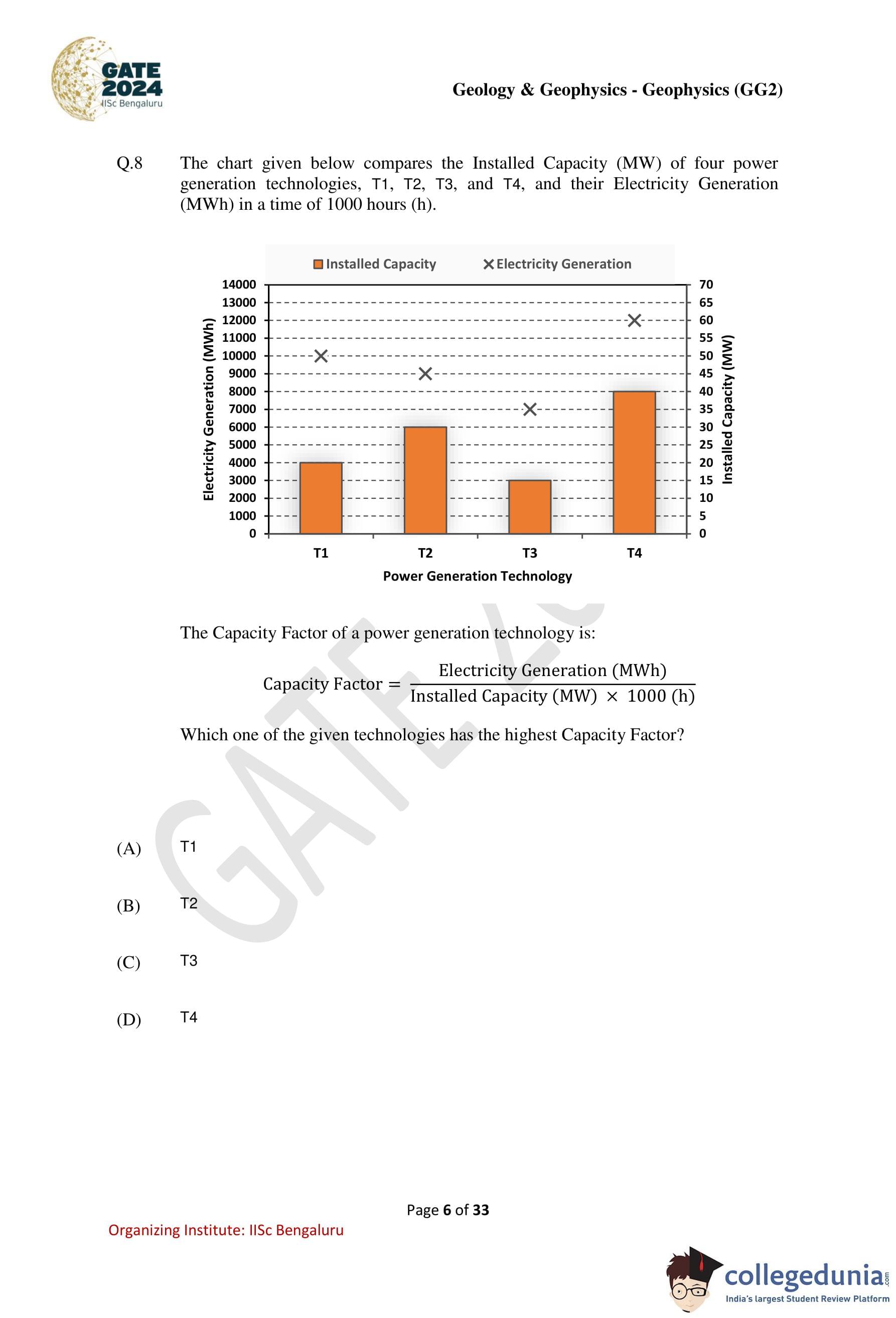
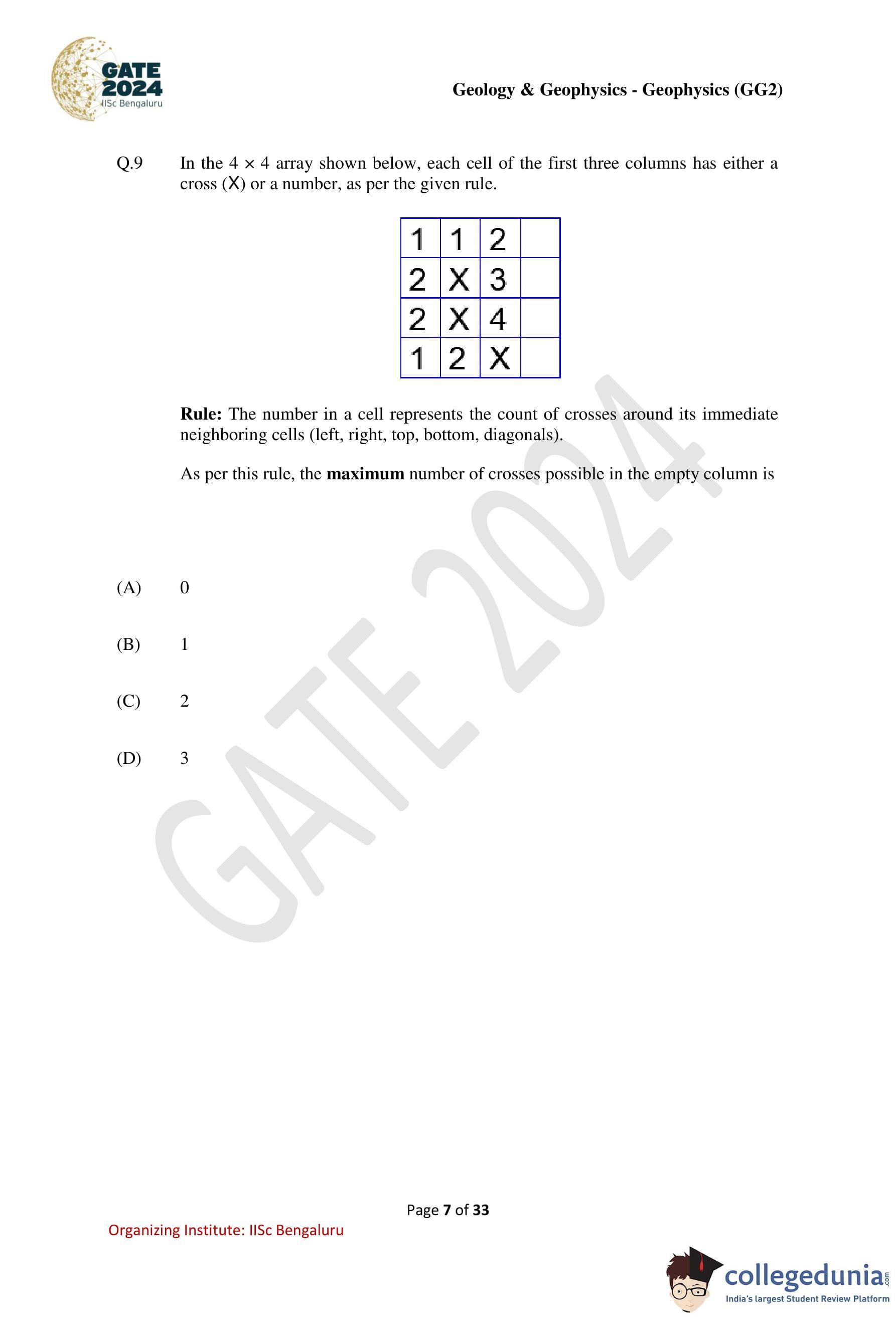
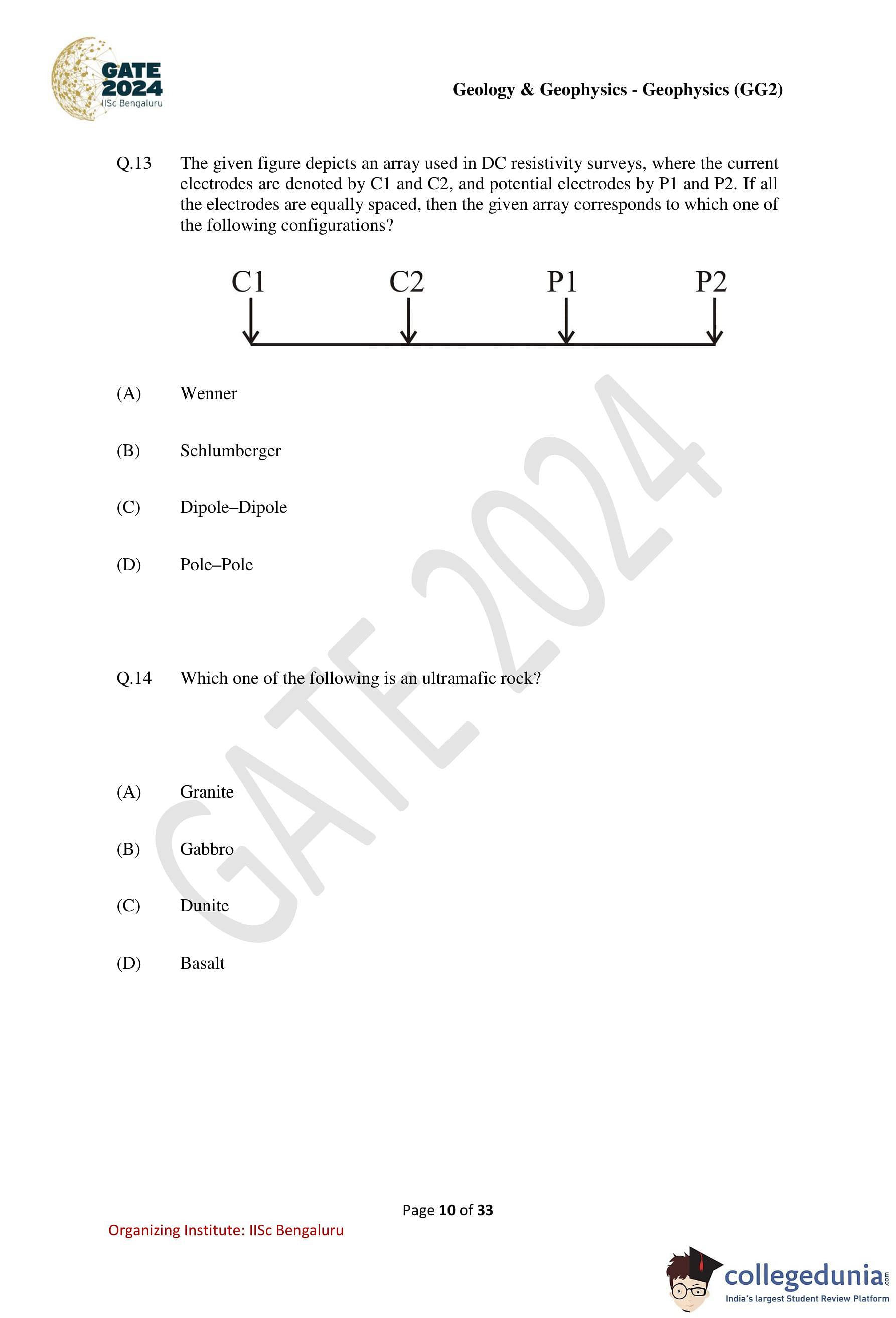
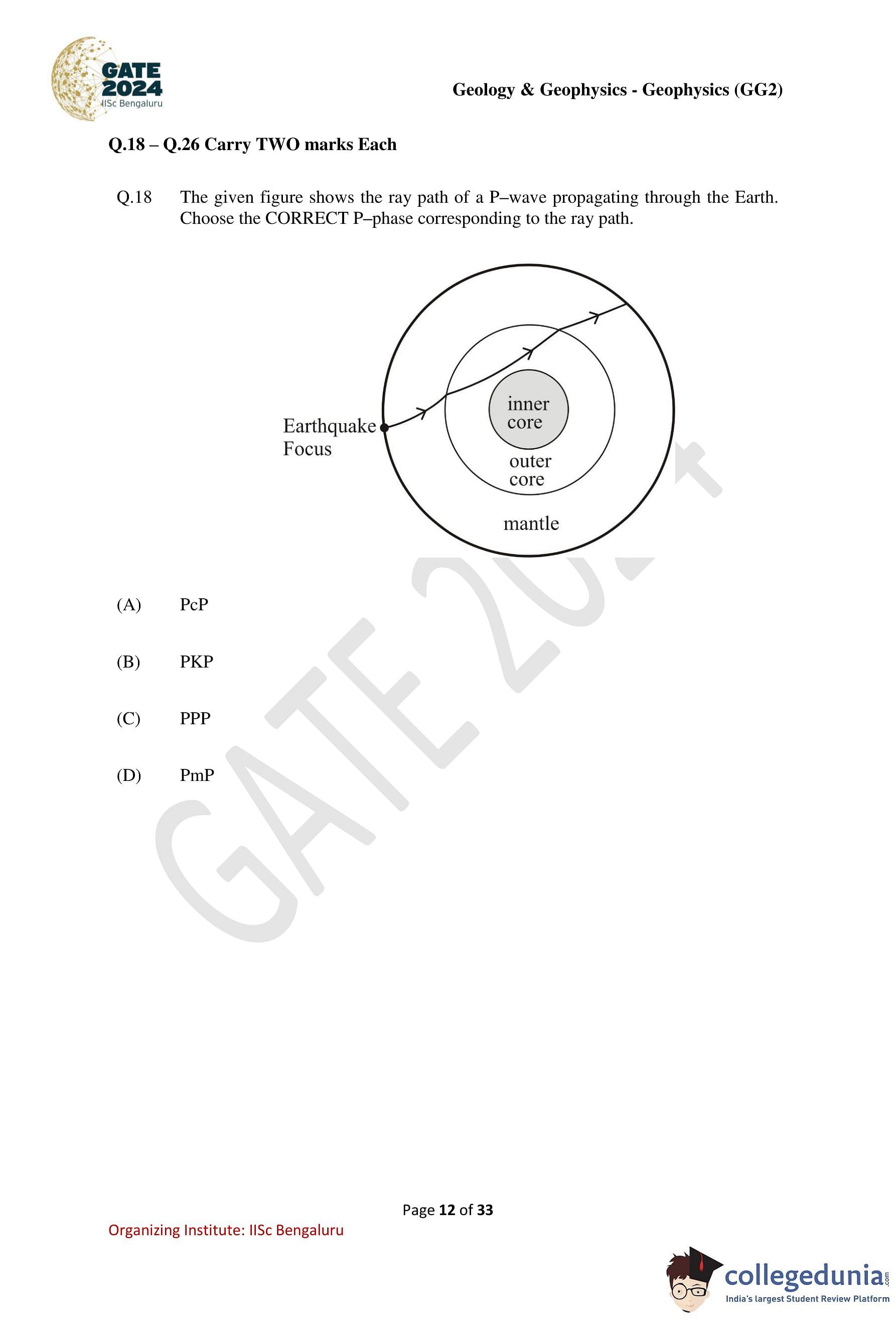

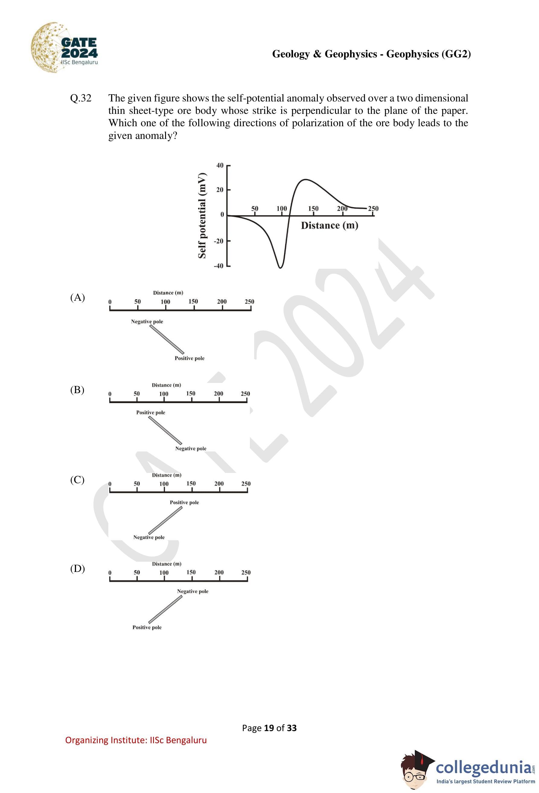
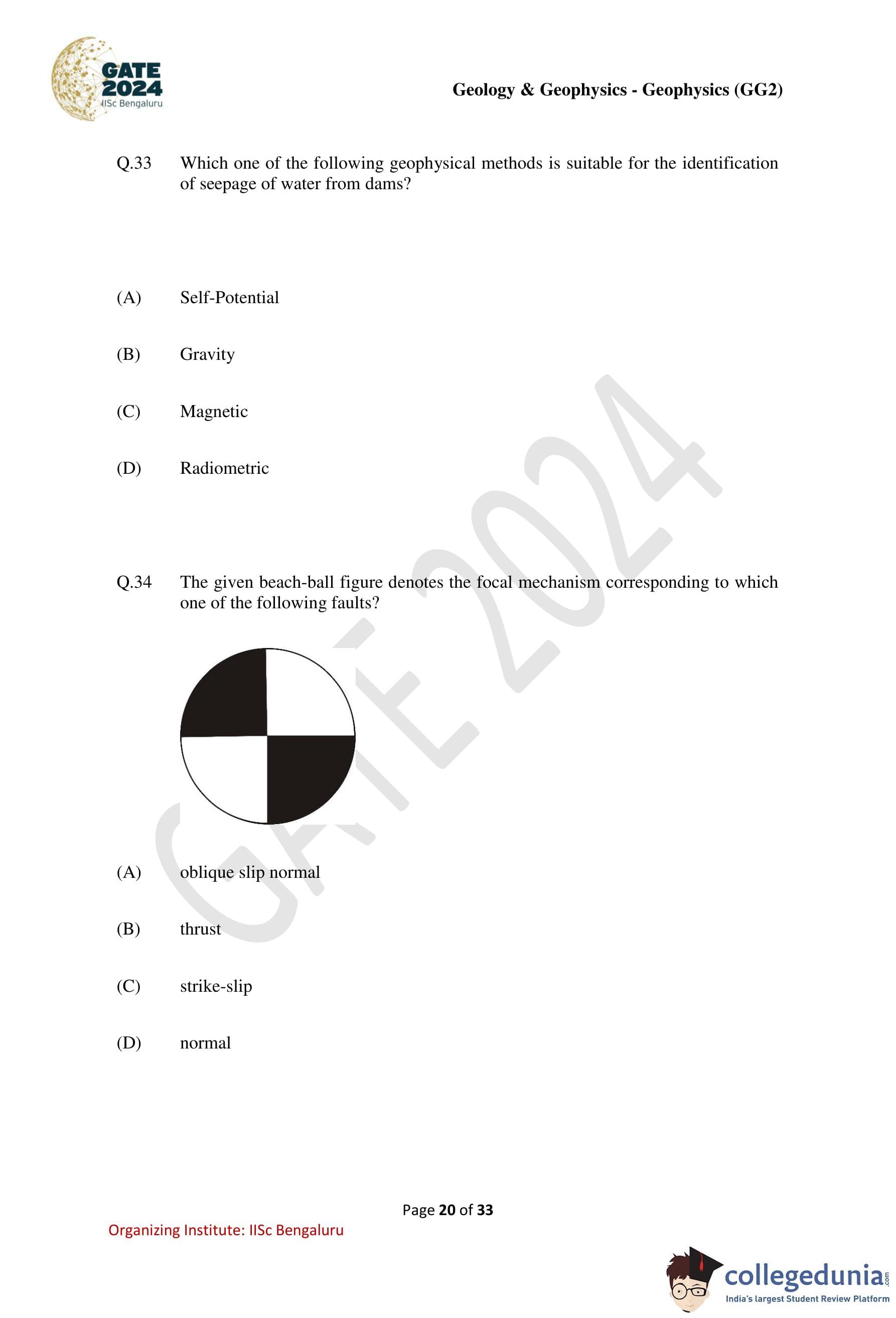
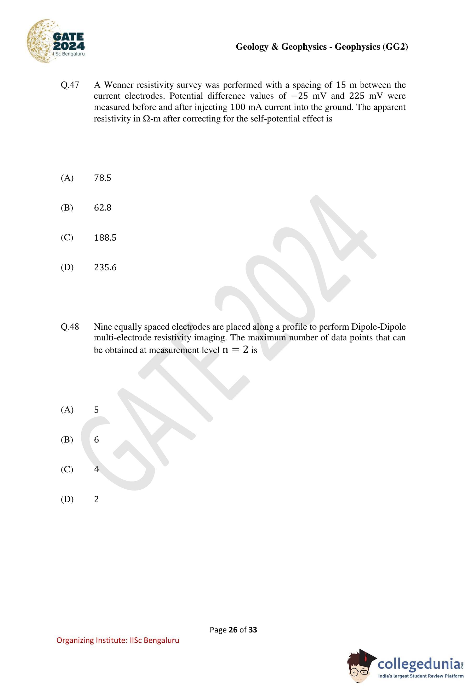
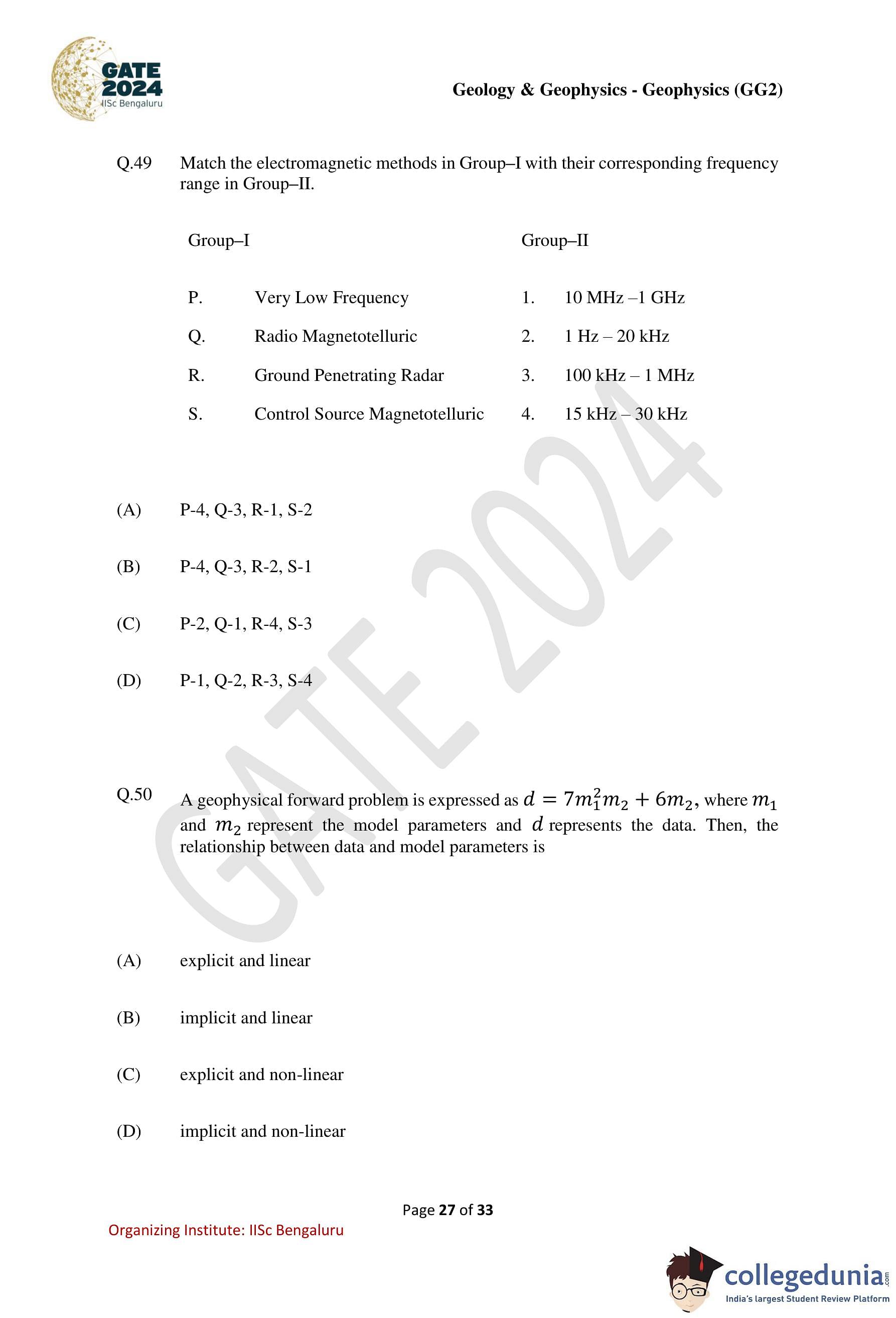
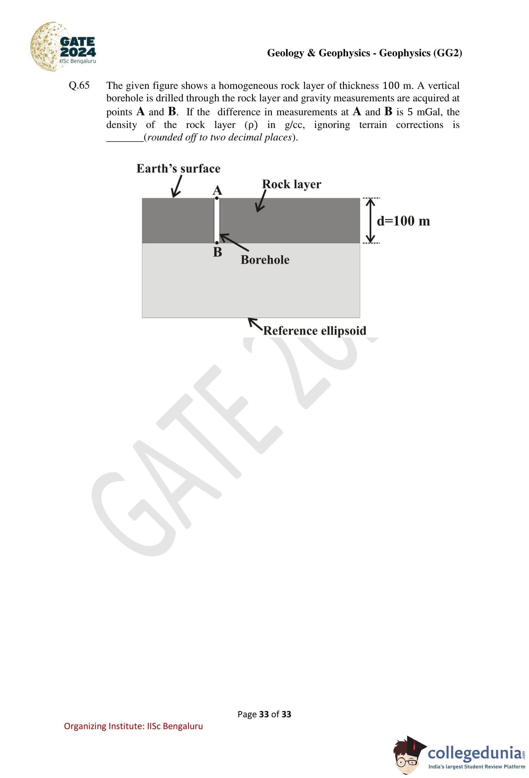
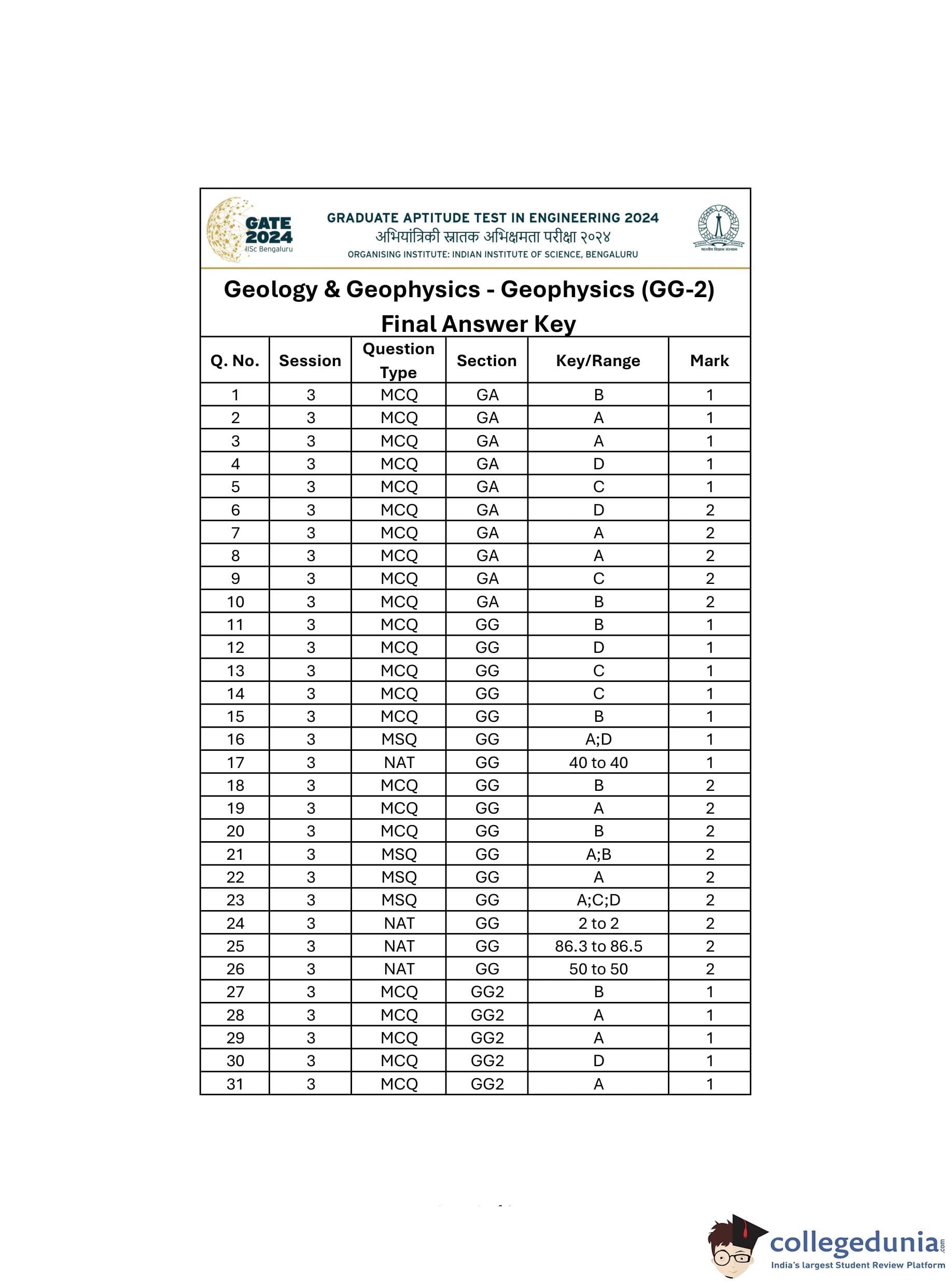
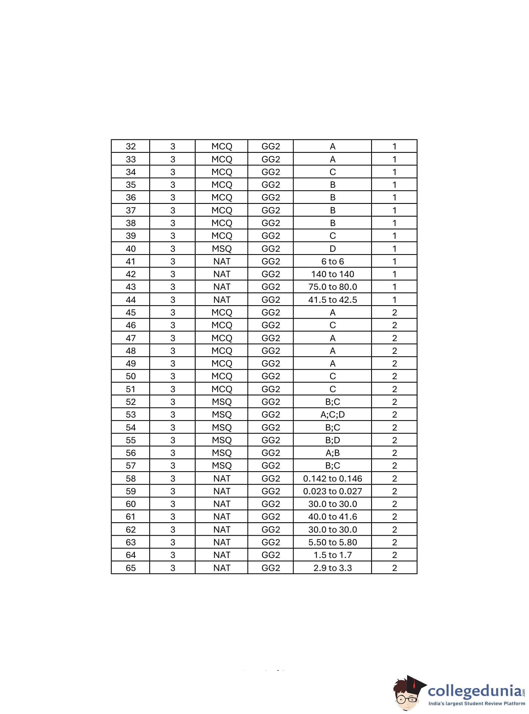
Also Check:


Comments